In this post I’m going to go through the kernel trick and how it helps or enables various tools in statistics and machine learning including support vector machines, gaussian processes, kernel regression and kernel PCA. This is going to be a bit of a long one, I’ll probably split it up later but for now … sorry? {}

Table of Contents

• Linear Methods
  • Fisher Linear Discriminatory Analysis (KDA I)
  • Support Models (SVM I)
  • Ridge Regression (KRR I)
  • Principle Component Analysis (Kernel PCA I)
• Kernel Trick
• Awesome Kernel-Based Methods
  • Kernel Discriminatory Analysis (KDA II)
  • Support Vector Machines (SVM II)
  • Kernel Ridge Regression (KRR II)
  • Kernel Principle Component Analysis (Kernel PCA II)
• Gaussian Processes
• Gallery of Kernels
• Conclusions / Pros and Cons of Kernel Methods
• More Examples

Prerequisites

Sorry in advance if this post isn’t as accessible as my other ones. Since it’s quite a long one I’m going to presume some knowledge going in. Primarily,

• dot products + inner products and that one is a subset of the other
• Projections on to lines and planes from a Linear Algebra perspective
• Lagrange Multiplier problems
• and as usual, basic calculus (primarily multivariable derivatives of and with scalars and vectors) and some matrix algebra.

And yes all the links are Wikipedia, they’re good pages. And if Wikipedia is there, why not use it.

General Resources

• Cambridge series in statistical and probabilistic mathematics: Asymptotic statistics series number 3
  • Sorry that this one isn’t open access, but I was lucky enough to have access through my institution and it’s great. If you have institutional access or can afford it I’d highly recommend it (as of 2025)
• High-Dimensional Statistics - A Non-Asymptotic Viewpoint - Martin J. Wainwright
  • Also sorry that this one isn’t open access either, same situation as above.
• Jeff Calder: “An intro to concentration of measure with applications to graph-based l… (Part 1/2)” - Institute for Pure & Applied Mathematics (IPAM)
  • Not directly relevant, but is something to think about with all the talk of high-dimensional statistics on this page
• Steinwart - “Support Vector Machines”
• Rasmussen - “Gaussian Processes for Machine Learning”

Intro

The goal of this blog post is to make you the reader aware or appreciate more kernel-based methods. For that I’m going to structure the post as 1. Some linear-ish methods that show promise for being even better in non-linear contexts but seem computationally expensive, 2. How the kernel trick allows us to get around this computational bottlenecks, and finally 3. The final form of the kernel-based methods and those that simply don’t work without it (GPs).

I’m not going to presume knowledge of these methods beforehand as much as possible, but I am going to do a bit of a whirlwind tour, so if any of them seem interesting to you and you don’t think the level of detail I provide is good enough, I’ve tried to include some independent resources for each that maybe will provide another perspective or more detail for every sub-section (the ‘Resources’ sections).

And as should be stated in all of my posts (but to be clear isn’t), I use notation through which I understand everything or simply want consistent notation throughout a given post so will likely differ from standard notation for a given topic(s). If you think I should make a given idea or object different notation either to make it clearer or because it’s simply incorrect please email me at lc[LastNamelowerCase]@[googleAddress].com or [FirstName].[Lastname]@[my institution].edu

Linear Methods

Fisher Linear Discriminatory Analysis (KDA I)

Resources

• StatQuest: Linear Discriminant Analysis (LDA) clearly explained.
• Linear discriminant analysis - Wikipedia
• Basics of Quadratic Discriminant Analysis (QDA) - Kaggle
• FISHER’S DISCRIMINANT ANALYSIS - Sanjoy Das
• The Use Of Multiple Measurements In Taxonomic Problems - Fisher
• Kernel Fisher discriminant analysis
  • Has a nice concise section on the linear case

The Gist

Fisher Linear Discriminatory Analysis or simply FLDA¹ is a supervised method (meaning we know the class labels) for creating a linear projection (single value in 1D, line in 2D, plane in 3D) that separates two or more classes of objects. Here we will focus on the separation of just two classes.

The key idea behind FLDA is that you wish to construct some linear combination of the input variables to demarcate the two classes that you project the objects onto. You do this by 1. maximising the distance or variance between the two groups on the projected space and 2. minimising the variance of each group in this space. Below are some examples of this in action before we get into it to emphasise that both conditions must be satisfied to get good discrimination.

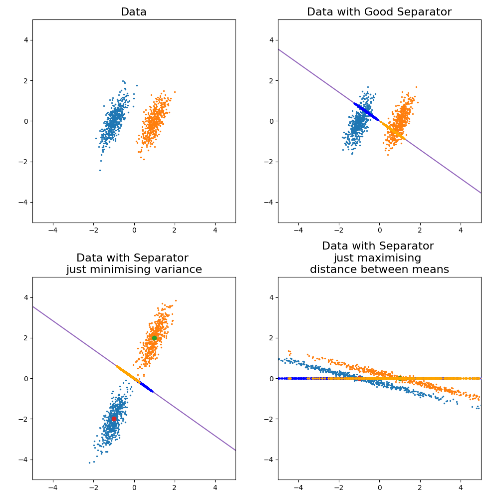
In a very non-statiscian way I’m just going to throw the formula here and leave the derivation to another day (as I will do for quite a few things in this post).

The \(\vec{w}\) is a vector in the direction of line (or linear operator on variables for generality) that is used in the above as a projection operator, to note the statistical measures on the line. There is any analytical solution to this where,

Where the solution as increases or decreases in the magnitude, the direction vector still return the same line object. For the sake of a cool gif and for later on when we generalise this method, let’s look at how it looks when you try to optimise for \(\vec{w}\) and compare it to the exact solution above.

Let’s compare the optimisation result to my “guesses” above.

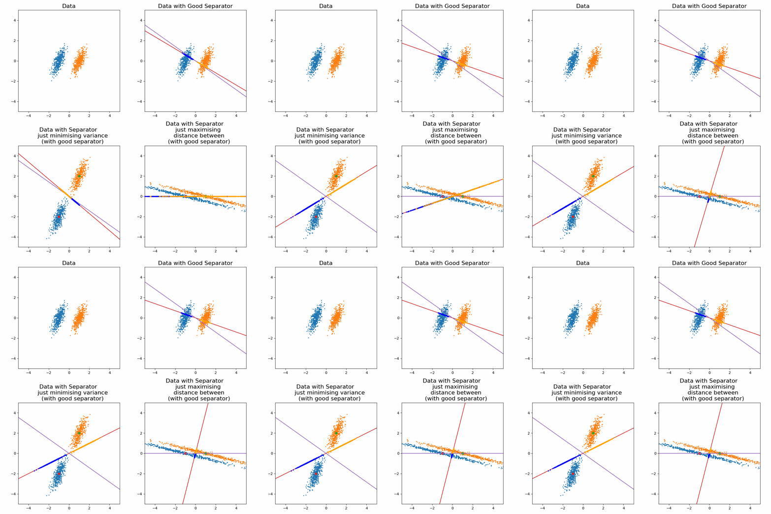
And voila, my good guess wasn’t as good as I thought and my bad guesses were in fact … bad.

Switching gears a little bit, let’s simplify the problem and look at a 1D example, still 2 groups.

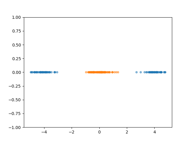
Now, if we wanted to do FLDA, we can only create a single value to discriminate the groups. But no matter what value you pick, there is no single value that will perfectly discriminate the groups despite it visually looking very simple.

The trick is to² increase the dimension of the space, projecting the 1D dimensional data \(x\) into two dimensions where the second is \(x^2\).

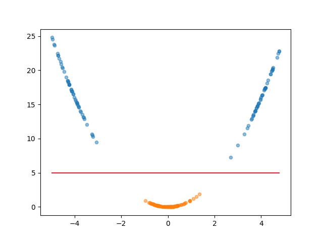
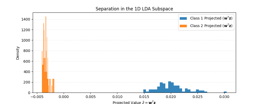
In this space, it is an extremely simple task of constructing a linear combination of the variables (again just a line in 2D) that the data can be projected onto and be separated. Additionally, I’ll start plotting the decision boundary that this implies in the space, which both separates the data and shows what direction it needs to go to be projected onto the LDA space.

Mathematically, nothing really changes compared to before, but we can slightly rephrase it so that it’s easier to generalise to more dimensions.

So we go back to maximising the variance \(B\)etween the class and \(W\)ithin for data from group 0, \(x_0\), and group 1 \(x_1\).

Okay great now we can separate groups like that. But let’s add one more cluster of points, and project it into the same space

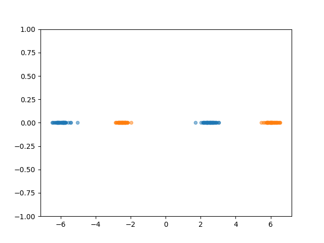
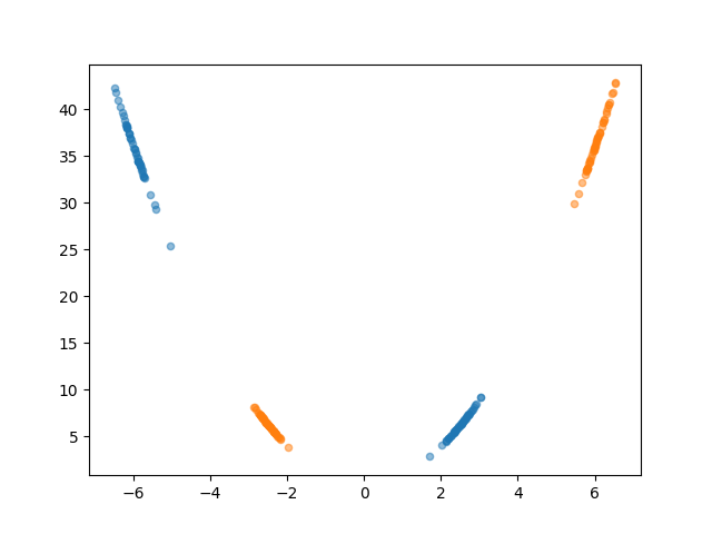
The projection doesn’t really help us again, no matter what line you pick you can’t separate the groups. But what if we keep going? Projecting it into the 3D space with the third dimension being \(x^3\) gives us the plot below (interactive).

Where we’ve constructed the line and planar boundary which are just linear combinations of the variables we are considering \(x^3\), \(x^2\) and \(x^1\). I like to think of the plane here as the surface over which the samples radially converge onto the LDA projection.

You can see that increasing the dimensionality allows us to separate groups with more complicated morphologies, or to handle morphologies were we don’t know what projection will work a priori, but the computational cost quickly explodes in the case of even low dimensional data. e.g. If our data is just two dimensional \(x\) and \(y\) then the “cubic” projected space would contain \([1, x, y, xy, x^2, y^2, xy^2, x^2y, x^3, y^3]\) (with the 1 included to highlight how the lower dimensional contributions stick around). So we went from \(\mathbb{R}^2\) to \(\mathbb{R}^9\) (excluding 1) and you can imagine how bad this would get in the case of 4D data like \(x, y, z\) and time, and a degree 4 polynomial projection … but note that all the optimisation and the projections only go through dot products …

Here’s the code for calculating the FLDA projection cost function for an arbitrary set of samples and dimensionality.

def calculate_scatter_matrices(samples1: np.ndarray, samples2: np.ndarray):
    mean1 = np.mean(samples1, axis=0)
    mean2 = np.mean(samples2, axis=0)
    
    N1 = samples1.shape[0]
    N2 = samples2.shape[0]
    N_total = N1 + N2
    total_mean = (N1 * mean1 + N2 * mean2) / N_total

    centered1 = samples1 - mean1
    S1 = np.dot(centered1.T, centered1) 
    
    centered2 = samples2 - mean2
    S2 = np.dot(centered2.T, centered2) 
    S_W = S1 + S2
    
    diff_mean1 = (mean1 - total_mean)[:, np.newaxis]
    diff_mean2 = (mean2 - total_mean)[:, np.newaxis]
    S_B = N1 * np.dot(diff_mean1, diff_mean1.T) + N2 * np.dot(diff_mean2, diff_mean2.T)

    return S_W, S_B


def lda_objective_function(w, S_W, S_B):
    
    numerator = w.T @ S_B @ w
    
    denominator = w.T @ S_W @ w
    
    J_w = numerator / denominator

    
    return -J_w

Linear Support Vector Machines (SVM I)

Resources

• Support Vector Machines Part 1 (of 3): Main Ideas!!!
• 16. Learning: Support Vector Machines - MIT OCW
• CS229 Lecture notes - Support Vector Machines

The Gist

Support vector machines are another supervised linear method where we want to construct some way to separate data, except unlike FLDA where we want to develop the projection, instead, we want to figure out the boundary, then we can figure out the projection later if we want. I’m just gonna come out and say that I’m stealing most of my examples from the MIT OCW lecture above.

The use case is similar to before except I want to raise two particular very similar issues in FLDA. Let’s say we have the two datasets below.

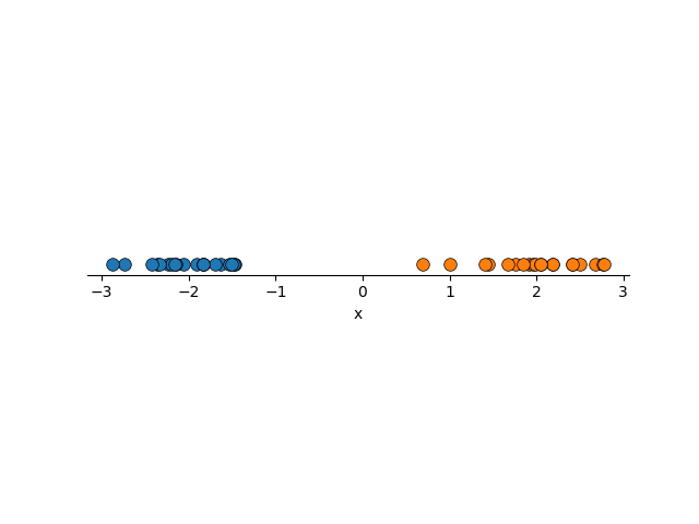
Using FLDA we would construct boundaries similar to the below, and we want to introduce some new data that is unlabelled.

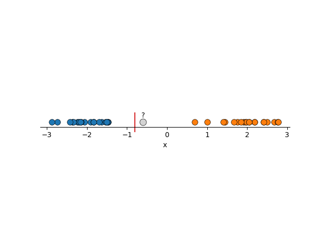
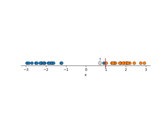
In both cases, it seems obvious to us what the new points should be labelled as, but using two lines that are perfectly fine under FLDA, both would be mis-characterised. The solution, is to 1. Maximise the region around the boundary and 2. not care so much about mis-labelling some points in our training data. Using these principles you can imagine that we would get something more reasonable.

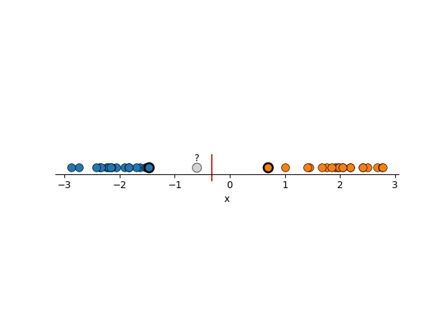
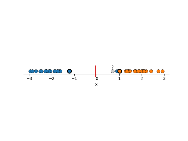
To me, this seems much more reasonable. And you might have noticed that I’ve highlighted a couple points, reason being that the decision boundary that is constructed here is basically just the average position of these two points. Removing any other points wouldn’t make the boundary any better or worse (except maybe the blue point in the right example). We call these points support vectors and it’s where the name for Support Vector Machines come from. I’ll circle back to why this is in a bit.

Before jumping into Support Vector Machines, instead I want to start with Support Vector Models and how they are constructed. (From here I’m pretty closely “following” the MIT OCW lecture.)

To make the visualisations less boring let’s go back to 2D. I spent too much time coming up with some useful randomish values.

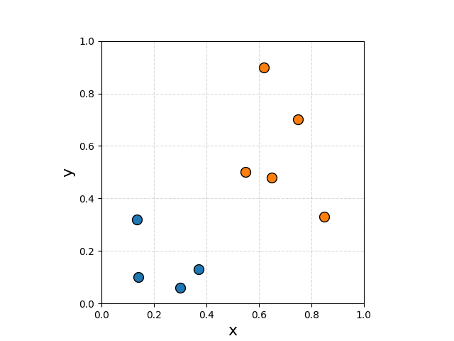
If we wanted to create a boundary that is maximally wide that distinguishes the two classes it would look something like this.

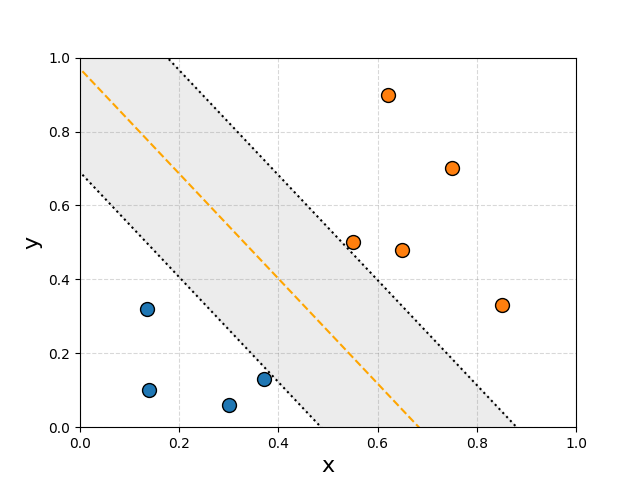
The region would then be defined either by the direction vector of the orange/yellow dashed line or the normal vector. For now let’s say we want to use a normal, the length doesn’t matter, just the direction. This then lets us very nicely define whether a point \(\vec{x}\) is contained in the region by a projection onto this line \(\vec{w}\cdot\vec{x} + b\). We define the yellow line to be the 0 point on the projection \(\vec{w}\cdot\vec{x} + b = 0\), and the boundaries to correspond to \(\pm1\), \(\vec{w}\cdot\vec{x} + b = \pm 1\).

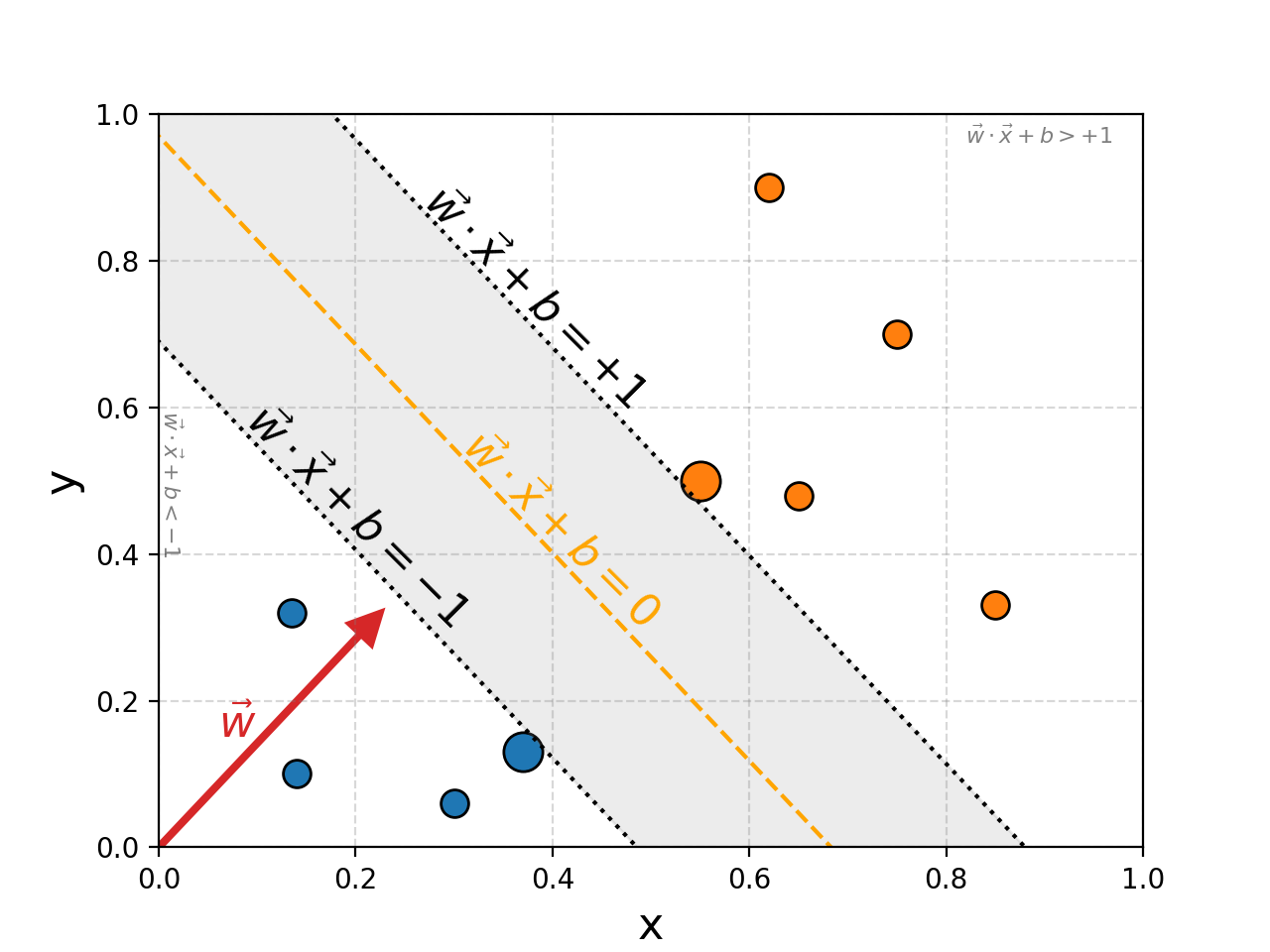
The area above the region will then be larger than \(1\), \(\vec{w}\cdot\vec{x} + b > 1\), and below will be less than \(-1\), \(\vec{w}\cdot\vec{x} + b < -1\).

Okay, so we have the kind of goal we want, the question is how do we mathematically recover it (can’t just do it ‘by’ eye in 4D, or 16D for that matter). Let’s outline what we know.

We know for points from group 1/orange points, that they evaluate to larger than or equal to \(1\),

and for points from group 2/blue points, that they evaluate to less than or equal to \(-1\),

Keeping track of two separate expressions like this is kind of annoying though. So let’s introduce a mathematical ‘nicety’ where we label points from group 1 with \(+1\) and those from group 2 with \(-1\). Hence, for all points (\(\forall i\in [1, N]\) \(N\) being the total number of points),

That’s better! Now, the single mathematical object that we wanted to maximise was the width of the region.

The width of the region is dictated by the support vectors that I’ve highlighted with a ‘+’ for group 1 and ‘-‘ for group 2.

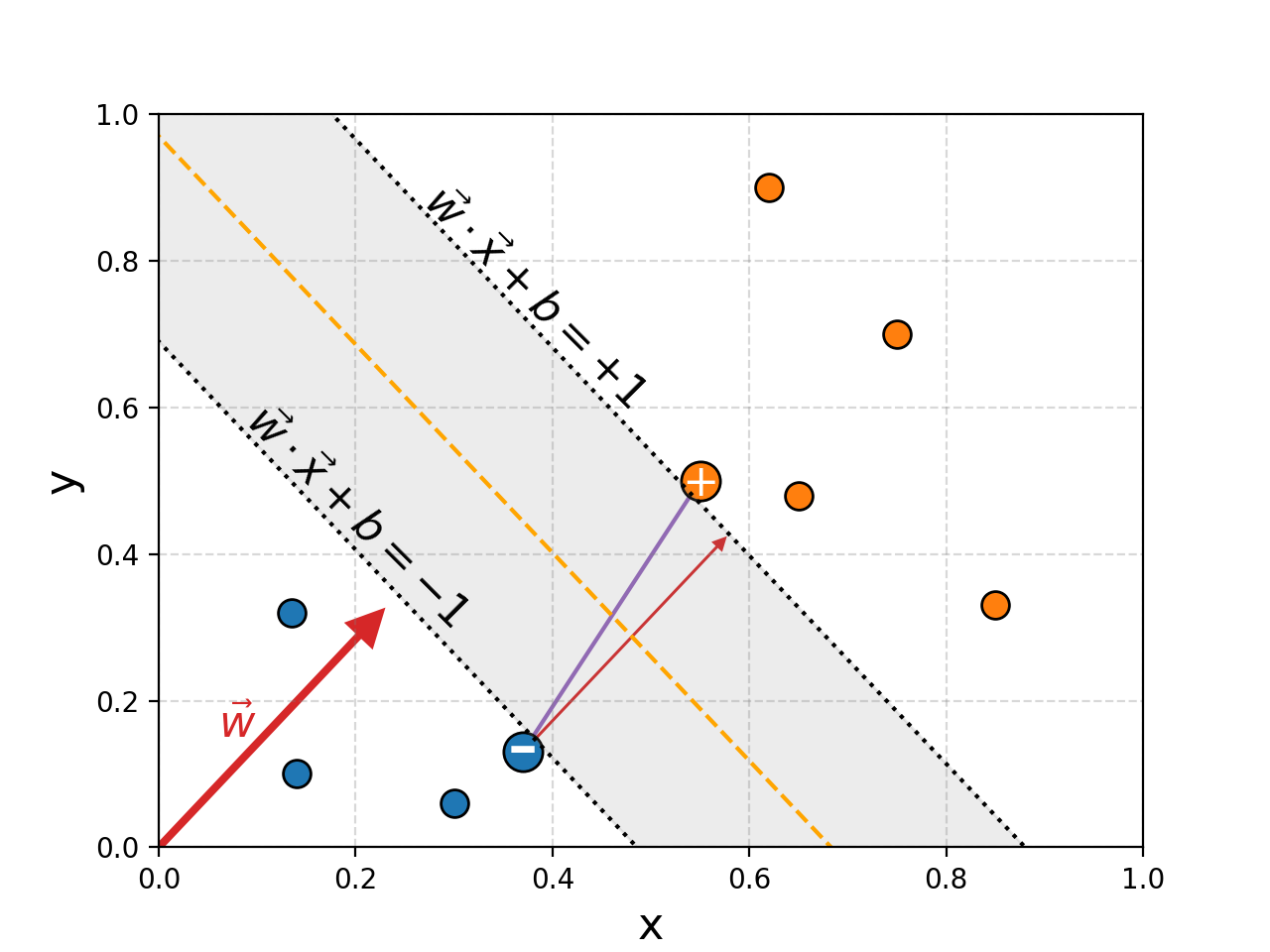
To figure out the width of the region we just need to project the distance between these two points and that of the perpendicular direction vector defining the region, this is show with a smaller red arrow in the above figure. It’s defined by a simple dot product as well (these dot products seem to be showing up a lot in this blog (hint hint)) with the normalised direction vector.

With a bit of algebra, and using the fact that the points lie at the lines at which \(\vec{w}\cdot\vec{x}_+ + b = +1\) and \(\vec{w}\cdot\vec{x}_- + b = -1\) to go from line 2 to 3.

So the goal is to maximise \(\frac{2}{\vert\vert\vec{w}\vert\vert}\), which is equivalent to maximising \(\frac{1}{\vert\vert\vec{w}\vert\vert}\), which is equivalent to minimising \(\vert\vert\vec{w}\vert\vert\), which is finally equivalent to minimising \(\vec{w}^2\), cool!³. But now instead of us wondering what the width is, we’re wondering what \(\vec{w}\) is…

From here we view the problem a little differently, we have an object that we wish to minimise, \(w^2\), subject to a bunch of constraints, \(y_i(\vec{w} \cdot \vec{x}_i + b) \geq 1\), … sounds like a Lagrange Multiplier problem. Jumping straight into it.

In \({\color{blue}\textrm{blue/left term}}\) is the thing we are minimising, and in \({\color{red}\textrm{red/right term}}\) are the constraints with \({\color{red} \alpha_i}\) the set of lagrange multipliers. The cool thing here is that \(\vec{w}\) is just some linear combination of the points in the two sets! That’s it, no weird error functions or logs or exponentials, just a simple linear combination (one might even say dot product).

Then we do the same ol’ song and dance. Taking derivatives with respect to \({\color{red} \alpha_i}\) just gives us back our constraints, so focusing in on \(\vec{w}\) and \(b\).

Highlighting the important bits in green and purple. We can then sub this back into our loss \(L\)/lagrange equation.

Staying to the theme, the final calculation comes down to a simple dot product between the data points \(\vec{x}_i \cdot\vec{x}_j\). So unlike FLDA we don’t have an analytical solution, but we do have a function that we can optimise.

The aim of the game is now to optimise over \(\alpha_i\) to minimise \(L\).

Translating this into the code.

def supportvecmodel_costfunc(alphavec, datavecs, labelvec):     
    K = np.dot(datavecs, datavecs.T) # wink wink
    
    alpha_y = alphavec * labelvec
    
    P = np.outer(alpha_y, alpha_y) * K
    quadratic_term = 0.5 * np.sum(P)
    
    linear_term = -np.sum(alphavec)

    cost = quadratic_term + linear_term
    
    return cost

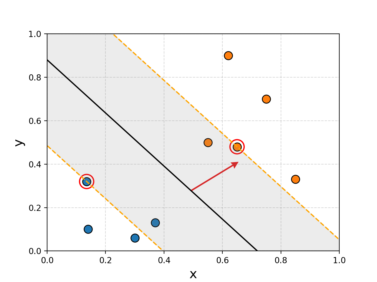
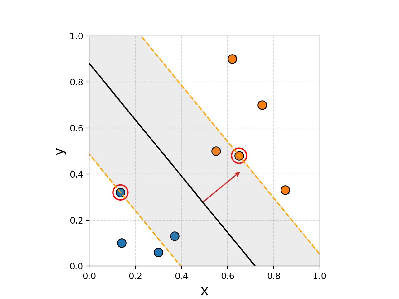
You can hopefully see that the margins are significantly wider despite not having 100% accuracy when discriminating between the two groups. This is a pretty simple example though, let’s see what it looks like when we increase the number of samples.

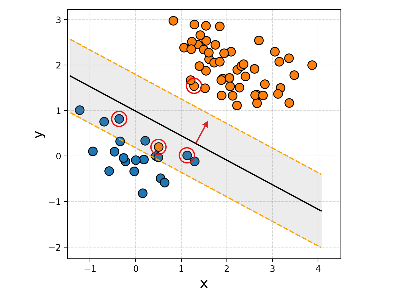
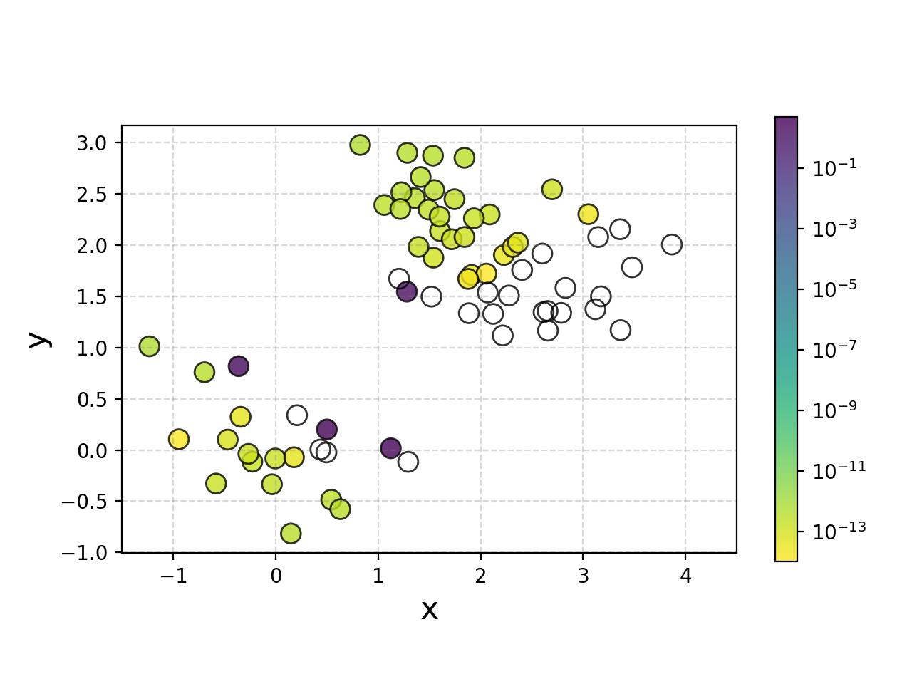
We can also plot the weights for how much each point is contributing to the decision boundary for fun, and broadly it makes sense.

So this is great, but as noted in the previous section, data isn’t always separated so nicely. For example…

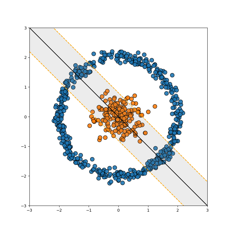
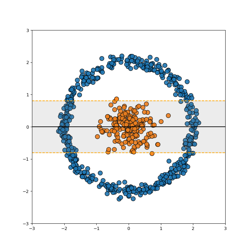
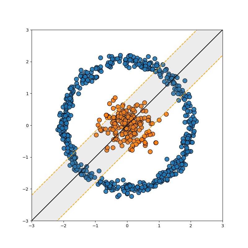
Well, we can use the exact same trick we used in the FLDA case, we add a dimension which is some polynomial combination of the variables (for those that already know where I’m going, this corresponds to a degree 2 polynomial kernel).

And to be clear, this uses the exact same math as above, just now \(x^2+y^2\) is another dimension in \(\vec{x}_i = [x, y, x^2+y^2]\) with the same ol’ dot products. This is great! Right? Well then what about this example?

It might seem a bit contrived but you could imagine a study where they’re looking at the interaction of two drugs. A little of both does nothing, a good amount of one and a lil of the other yields good outcomes, but too much of both leads to unwanted drug interactions and bad outcomes. The quadratic projection wouldn’t help here, and other low order polynomial projections likely wouldn’t either. So once again.

Ridge Regression (KRR I)

Resources

• Bayesian Linear Regression : Data Science Concepts - by my man ritvikmath
• Data analysis recipes:Fitting a model to data - ArXiV:1008.4686 - David Hogg, Jo Bovy, Dustin Lang
• Ordinary least squares
• Ridge regression
• Generalised Kernel Machines
• Gauss–Markov theorem
• Bias-Variance Trade Off
• Temperature and Ice Cream Sales Kaggle dataset by Raphael Manayon

The Gist

Switching gears, or more switching cars at this point, let’s talk about regression. Plain ol’ linear regression. You have a dependent variable, \(y\), an independent variable \(x\), a set of samples of each \(\{y_i\}\) and \(\{x_i\}\), and you believe they are related via \(y= \alpha_1 x + \alpha_0\) (excuse the pointlessly mathy way of describing things, it will be useful later).

This is exactly what I did in my first blog post but in that case I went straight into the Bayesian probabilistic route. If we just wanted a best fit however, we don’t need to go through all the effort.

We can just define a linear system of matrices. Defining,

Using the above⁴ with \(Y=[N\times 1]\), \(\vec{\alpha}=[P\times 1]\) and \(X=[N\times P]\) we can define the system as,

And that’s it. \(Y\) is called the regressand, and \(X\) the design matrix. The aim of the game is to just figure out \(\vec{\alpha}\) … but wait, sure I don’t need uncertainties on my final parameter values, but I should include the uncertainties on my data if I have them right?? That doesn’t show up in the above. Well for that I find it easier to actually go back to the probabilities.

If we’re assuming that our data is distributed according to some normal distribution like the following (assuming homoscedacity for simplicity),

then our system becomes,

Where \(\vec{\epsilon}\sim \mathcal{N}(0, \sigma^2)\). Splitting it up this way is pretty close to the reparameterisation trick where all the stochasticity has movied to \(\vec{\epsilon}\) now and \(X \vec{\alpha}\) is deterministic. But that’s just a fun little aside.

As people who are aware of full probability theory, or want to go about this a lil rigorously, we would then want to maximise the probability of our parameters,

i.e. We want to find the maximum a posteriori (MAP) estimate. As part of the bias-variance tradeoff, the more parameters we include the higher our accuracy (less bias) but we get less individual information on the parameters (higher variance). Additionally, we run the risk of overfitting.

The way that this is typically done is via regularisation on the parameters fitted, giving them a tendency to go towards 0, such that they only meaningfully contribute in the case where they really improve the fit. We can encode this as a prior on our parameters, that they are distributed according to a normal distribution with some variance \(\tau_j = \tau\). (further assuming that we just put the same regularisation on all of them).

Where I denote a vector full of ones that is the relevant length \(\vec{1}\), and when I need it the identity matrix as \(I\). We can thus write down our likelihood and prior, a value proportional to our posterior.

Where \(k\) is the length/dimensionality of \(\vec{\alpha}\), \(C_Y\) is the covariance matrix for our data \(Y\), which is just \(\sigma^2\) and \(C_\alpha\) is the covariance matrix for our parameters in our prior which is a diagonal matrix of size \(k\) which \(\tau^2\) on the diagonal. Simplifying the above,

Now because of numerical instability issues and many other reasons, we then take the log of this expression and reverse the sign.

Where \(C \in \mathbb{R}\) is some arbitrary constant relating to the normalisation. If we’re just wishing to minimise this expresion with respect to \(\vec{\alpha}\) we can drop all the terms that don’t involve it and multiply everything by the constant \(2\sigma^2\) setting \(\sigma^2/\tau^2 = \lambda\) to make the math nicer.

Which is just ordinary least squares with a \(L_2\) regularisation on the parameters⁵, or ridge regression. Note that the uncertainties only come through in how they influence the regularisation, which is because we assumed that they are shared the same noise variance.

What’s the point of all this if we aren’t going to use it though? Let’s look at the relationship between the Temperature and Ice Cream Sales Kaggle dataset.

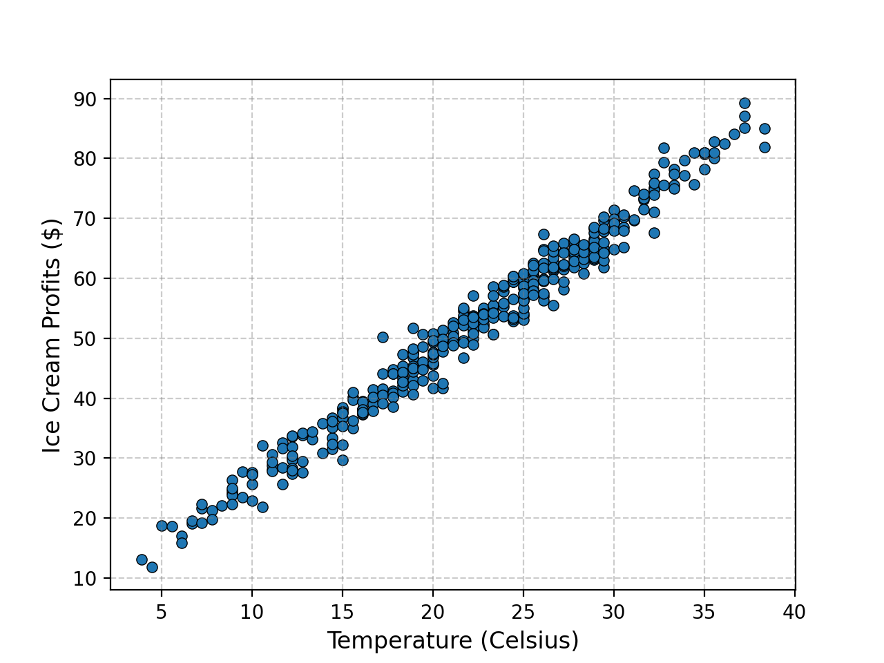
We can then see what the Ridge regression fit gives for different values of \(\lambda\) remembering that \(\lambda=0\) means no regularisation.

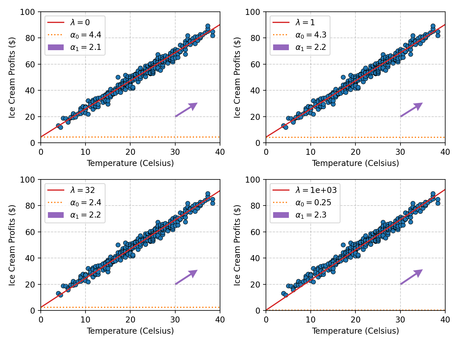
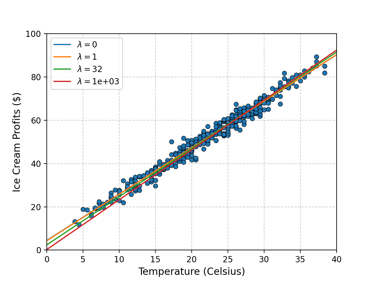
Here’s the code.

from scipy.optimize import minimize

linearY = data['Ice Cream Profits']
linearX = np.array([data['Temperature']*0 + 1., data['Temperature']]).T


def ridge_regression_cost(alpha, Y, X, lambdaval):
    return np.linalg.norm(Y - X @ alpha)**2 + lambdaval * np.linalg.norm(alpha)**2 


ridge_regression_cost(np.array([0., 2.]), linearY, linearX, 0.1)

result_dict = {}

for lambdaval in np.append(np.array([0.]), np.logspace(0, 3., 3)):
    linear_data_ridge_regression_result = minimize(
        ridge_regression_cost,
        x0 = np.array([0., 2.]),
        args = (linearY, linearX, lambdaval)
    )

    result_dict[lambdaval] = linear_data_ridge_regression_result.x

Alrighty, we have this very nice very automated way to perform our fitting. Let’s look at another example of the path of a basketball.

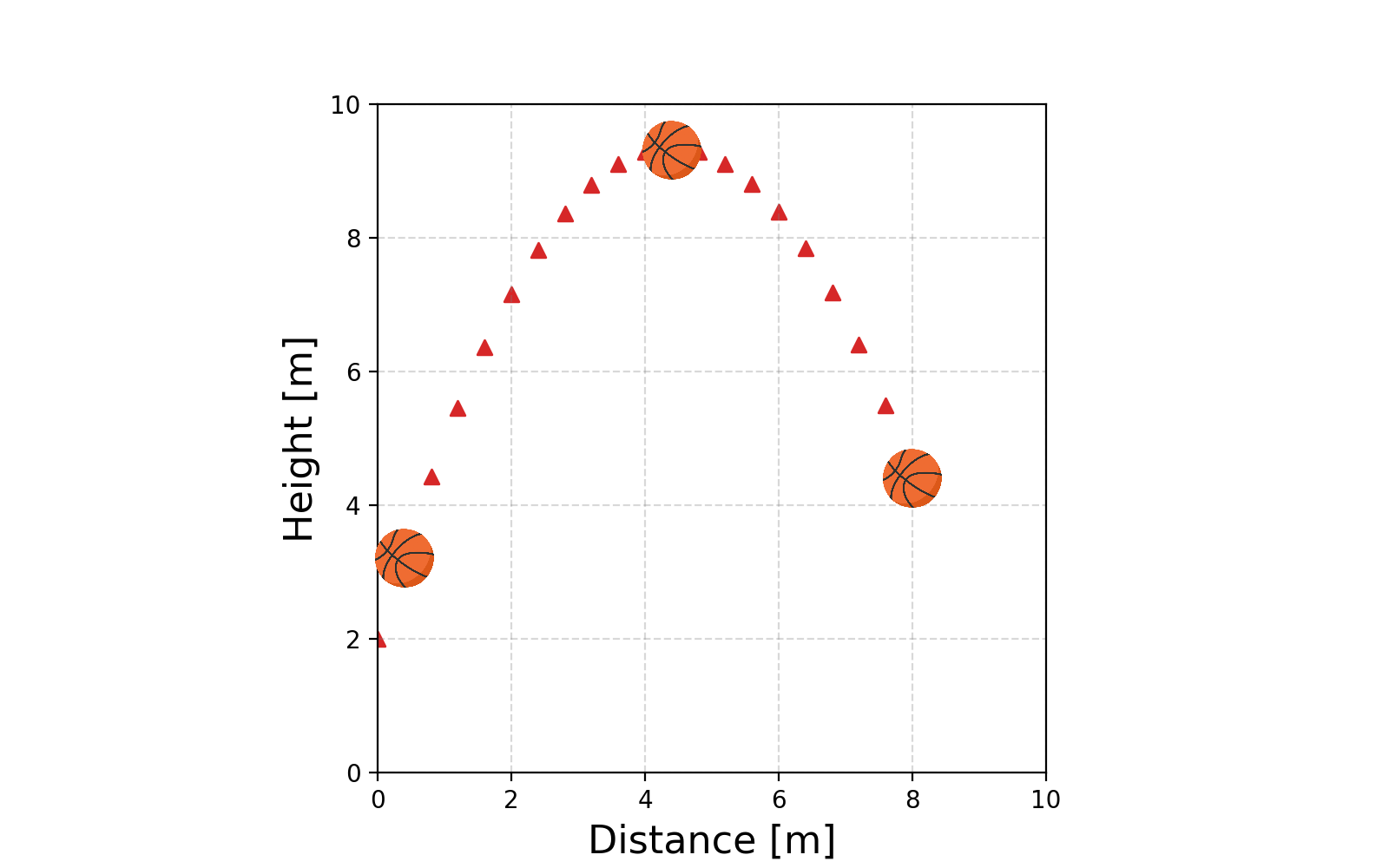
We know beforehand that the path will be parabolic and hence can’t be modelled linearly (or at least properly). And now we can’t use our very nice method any more 😢 … or can we?

We employ the exact same trick as in the previous two sections, particularly on \(x\). We pretend that we have a new variable, that is really just \(x^2\), and then fit a straight line in that space (everything is just dot or matrix products), which will be equivalent to fitting a polynomial, but to the framework, it’s still just fitting a straight line! So now our data looks like.

Let’s look at the data in the project space.

Wait, that still doesn’t look linear? What’s going on? Well that’s because the problem is linear with respect to \(\vec{\alpha}\) not \(X\) still. The linear object we are fitting is closer to plane within which the curve we want is contained, and more specifically the region with the constraint that \(X_1 = X_2\). Let’s look at some results of the fitting (same code).

We can also look at what these look like in the original space.

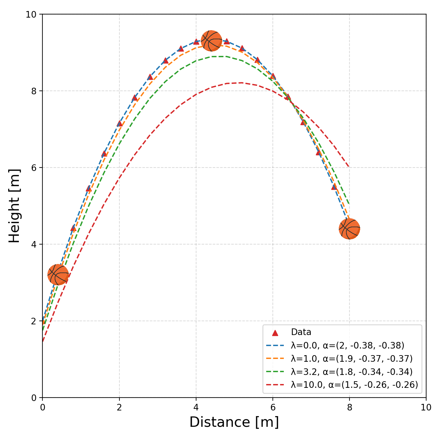
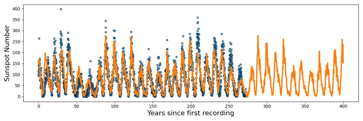
We can see that as the regularisation tightens, or we increase \(\lambda\), the constant term is particularly being penalised. That’s great, but again, we were helped out by knowing what form of equation to expect. Additionally, what if something was periodic like this sunspot data?

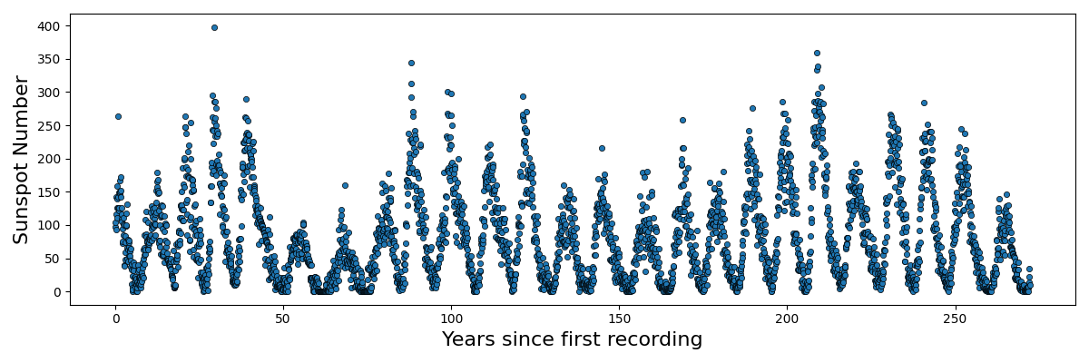
Do we just give up or…?

Principle Component Analysis (Kernel PCA I)

Resources

• Principal component analysis - Wikipedia
• Kernel Principal component analysis - Wikipedia
• Principal Component Analysis (PCA) | Dimensionality Reduction Techniques (2/5) - DeepFindr
• 19. Principal Component Analysis - MIT OCW
• Principle component regression - Wikipedia
• Principle component regression - Wikipedia
• Higher Order Reduced Rank Regression - ArXiv: 2503.06528

The Gist

To me Principle Component Analysis (PCA) is very similar to FLDA where we want to find a set of vectors that we can project the data on to best distinguish the data. PCA of course does it entirely differently (more robustly imo) but finding the direction(s) that maximise the variance in the given direction. The general process is as follows.

You have a set of n observations \(Z_i = [Z_i^1, Z_i^2, ..., Z_i^d] \in \mathbb{R}^d\) with \(Z_i^j \in \mathbb{R}^1\) with \(\mathbb{Z}^T = [Z_1, Z_2, ..., Z_n]\).

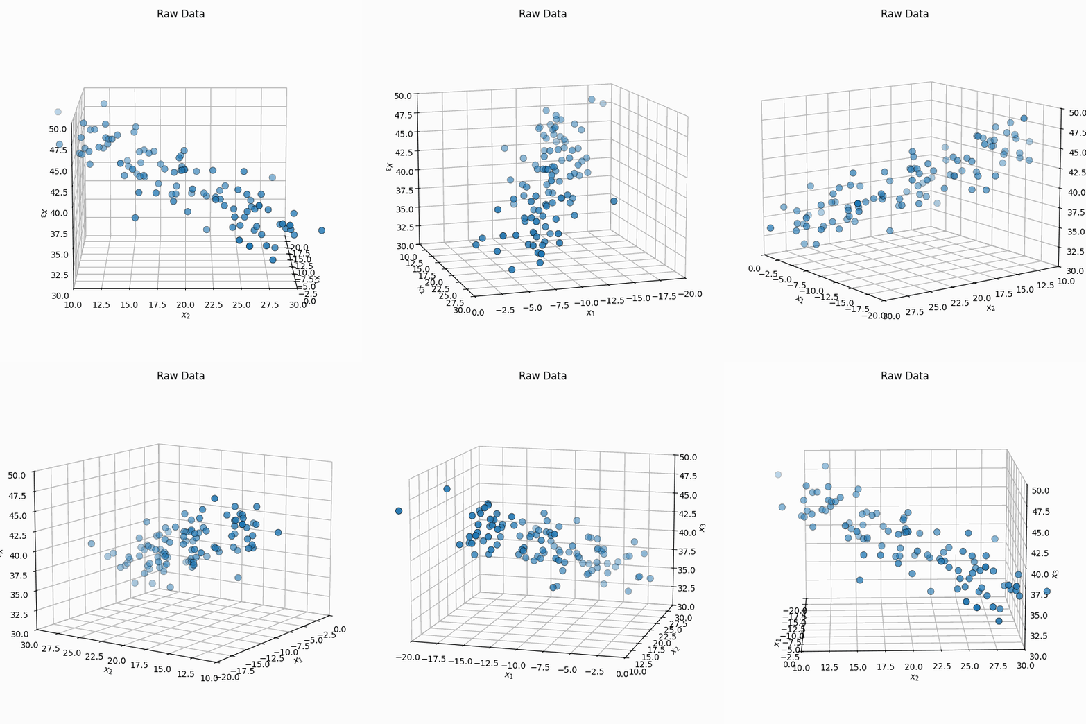
You shift it so that the mean is \(\vec{0}\), \(X_i = Z_i - \bar{Z}\) or \(\mathbb{X} = \mathbb{Z} - \frac{1}{n} \mathbb{Z} \vec{1}_n\) where \(\vec{1}_n\) is a vector of size \(n\) with every element equal to \(1\).

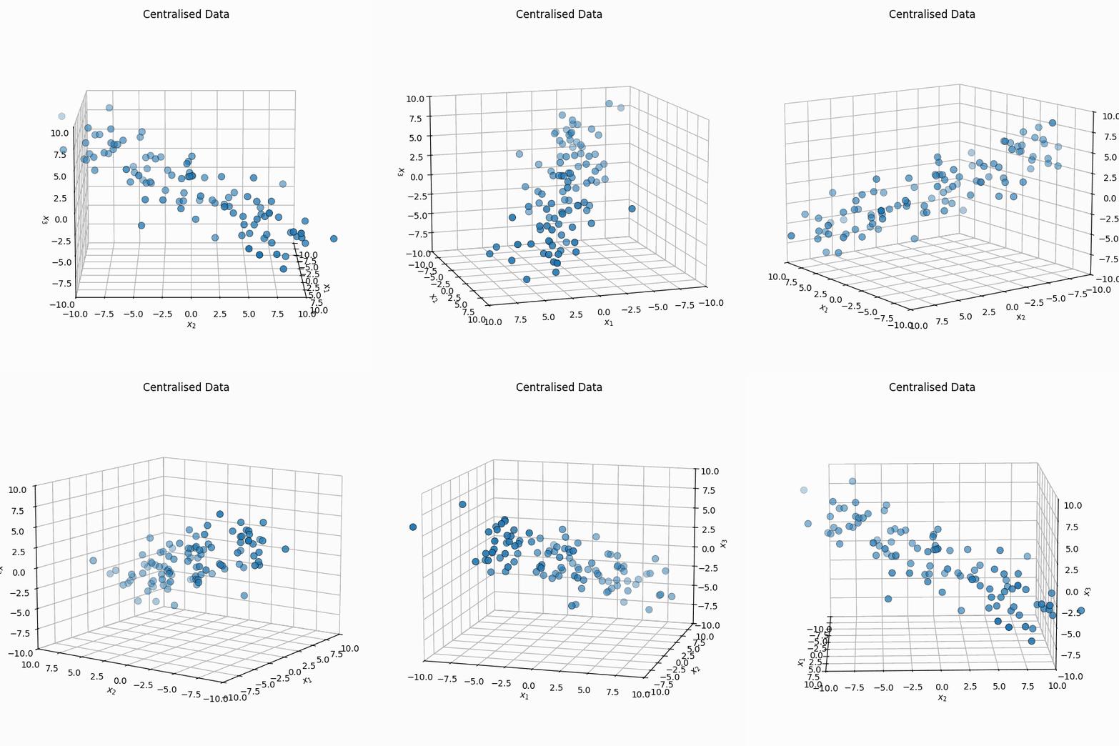
We then calculate the covariance matrix of the transformed data by first noting that the empirical covariance, \(S\), can be calculated as,

We can then perform Singular Value Decomposition which in this case is an eigendecompoisition as \(S\) is positive semi-definite and thus diagonalizable matrix. We know this as if we perform the operation for any vector in \(\mathbb{R}^d\), then we get the variance in that direction. i.e.

Hence, \(\exists P, D\) where \(P\) is orthonormal (\(P^T P = P P^T = I\)) and \(D\) is diagonal. Equivalently, this means we can represent \(P\) and \(D\) as,

where \(\lambda_1 > \lambda_2 > ... >\lambda_d \geq 0\) and

such that \(S = P^T D P\). The \(P\) matrix can be viewed as a projection operator that maps the centralised data into the space of eigenvectors, \(Y_i = P\, X_i\), within which data’s covariance matrix is the diagonal matrix \(D\).

We can also show that the variance in direction along which the variance is maximised, \(\vec{\mu}\) with \(\vert\vert\vec{\mu}\vert\vert = 1\), have a magnitude less than the largest eigenvalue \(\lambda_1\).

And by the definition of the eigenvector and eigenvalues, but just to go through the math explicitly,

Hence the eigenvectors are the ones that maximise the variance. So we skipped any optimisation (which wouldn’t be easy) by some simple linear algebra with the projection of new points just involving some dot products with the orthonormal bases. Assuming we have some quick method to calculate the eigenvectors and eigenvalues our mission is done!

For our data, the covariance matrix is as follows.

Then just blindly using the np.linalg.eig function we find the eigenvalues to be,

and eigenvectors to be

Let’s chuck this in an interactive plot to see how the eigenvectors look against the data.

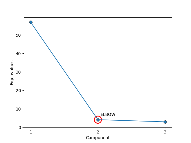
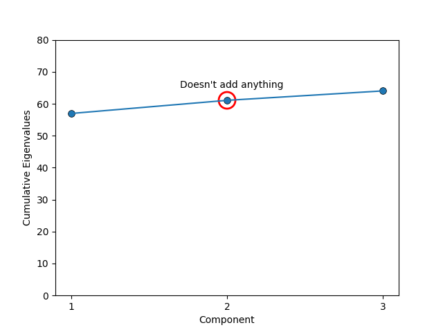
The process now gives us a whole set of vectors that we can use to reconstruct the data, but part of the point of this is to find the directions in the space of our data along which most of the information lies. So, we don’t actually want to keep all the vectors, but how many do we decide to keep? Typically, people just keep 1 to 3 (easy to visualise, and should explain most of the variation) but if one want to do this a little more rigorously we can use something called a Scree plot. Apparently named after its resemblance to the natural formation of broken rocks at the bottom of a cliff (image below).

All that it is though is that you plot either the eigenvalues in order (automatically descending) where you look for an ‘elbow’ where the magnitude of the components drop off or their cumulative values \(\lambda_1\), \(\lambda_1 + \lambda_2\), \(\lambda_1 + \lambda_2 + \lambda_3\), etc where instead you look for when the cumulation of the eigenvalues doesn’t significantly increase (basically the same thing).

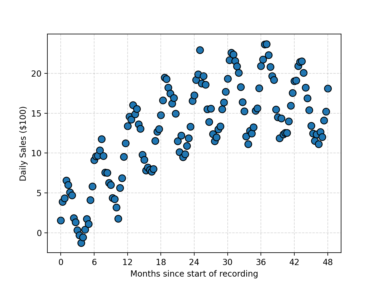
But let’s say that the data has some periodic component? e.g. In the below (fake) data, if we blindly apply PCA the amplitude of the periodicity would be included in the variance. Despite the data haing relatively low noise compared to the baseline sinusoidal signal with quadratic-like trend. At this point I’ll stop messing you around and just tell you the trick. (Unless you’re one of the unfortunate few to look at this before it’s finished.)

The Kernel Trick

Resources

• The Kernel Trick - Udacity
• RBF kernel as an infinite feature expansion - Andy Jones
• Lecture 15 of 18 of Caltech’s Machine Learning Course - CS 156 - Professor Yaser Abu-Mostafa
• Matthew N. Bernstein’s notes - The Radial Basis Function Kernel
• Support Vector Machines Part 3: The Radial (RBF) Kernel (Part 3 of 3) -StatQuest with Josh Starmer

The Gist

The idea that I keep coming back to in this post is that all of these methods on rely on just a series of dot products. I additionally showed that they all have (except PCA) much more generality and expressive power when we project our data into a higher dimensional space and use our linear methods there. But the grub was that even for low dimensional data, e.g. 4 for x, y, z and time, and just a degree 5 polynomial would have 59 columns in the design matrix (including constant). We then often perform an outer product so then we have to do \(59^2 = 3481\) calculations …. instead of 16 …. real expensive.

For example let’s say we have some 2D data,

that I then project into the higher dimensional ‘quadratic’ feature space (with some slight scalar adjustments compared to previous sections that wouldn’t make a difference to the end result),

We’ve also established that all of these methods simply compute the dot products between the vectors in this transformed space.

Then the magical thing is that this is equivalent to,

where \(K^{\textrm{poly}}_2(X^i, X^j)\) is referred to as a kernel function, more specifically a degree 2 polynomial kernel. Similarly we can look at two dimensional data,

and transform it into the cubic space,

the dot product between any two points in the this feature space would be,

For the second last line I’m just going to have to ask you to trust me if it doesn’t immediately seem right…

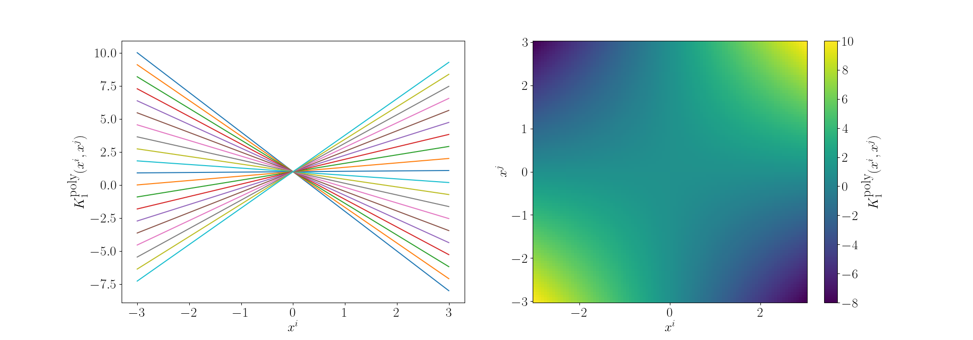
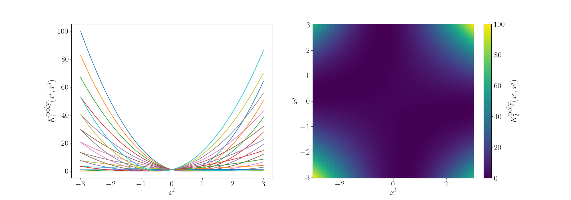
So the key point is that we can effectively do the calculations in the higher dimensional space without actually having to explicitly first transform our data into that space, as long as our kernel function is a valid inner product. What we can do in practice is store the values of the inner products between our data in what’s called a Kernel or Gram matrix. For now, we can just think of how the kernel’s behave in the context of the variables we give them. So we’ll plot the examples of the matrix for some 1D variable and just examine how the kernel behaves as a function of space.

For the degree 1 polynomial (directly below) we can see that the relationship between \(x^i\) and \(x^j\) is linear, as expected as we’re using a linear kernel. For a given \(x^j\) the value decreases as you move to the left and increases as you move to the right.

For the degree 2 polynomial (directly below) we can see that the relationship between \(x^i\) and \(x^j\) is quadratic. For a single value of \(x^j\) you can see that multiple values of \(x^i\) give the same inner product value. Meaning that if \(x^j\) was equal to 1 for example, \(x^i=1\) and \(x^i=-1\) would be equivalent from the eyes of the inner product.

And for the degree 3 polynomial (directly below) we can see that the relationship between \(x^i\) and \(x^j\) is cubic. And we can see more nonlinear behaviour pop up but the functions are monotonic so multiple values don’t give the same answer (for 1D, isn’t true for higher).

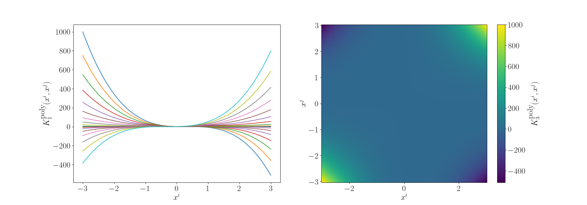
Not only can we implicitly transform our data into some finite dimensional polynomial space, we can also use kernels where the number of terms would be technically infinite.

e.g. the most commonly used kernel across disciplines is the Radial basis function kernel or simply the RBF kernel, defined as,

seeing as it has an exponential in it you can see that if we made the equivalent expansion as above that the series would be infinite. Setting the length scale \(\sigma\) to \(1\).

What the inner products between vectors would imply is pretty much a gaussian distribution with euclidean distance metric, or more simply, a quantity related to how close they are (that follows a gaussian distribution) or something like a weighted nearest neighbour model. If they’re far away from each other, the inner product is small, if they are near each other, the inner product is large. Spread out in a smooth manner due to the gaussian distribution.

Although the RBF Kernel works in infinite dimensions, we can visualise it’s truncated version to see how the behaviour arises. Thanks to Andy Jones for the heatmap code in their blog posts RBF kernel as an infinite feature expansion so I didn’t have to write it myself, please check it out if you have the time!

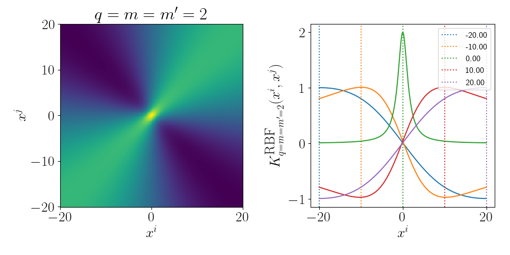
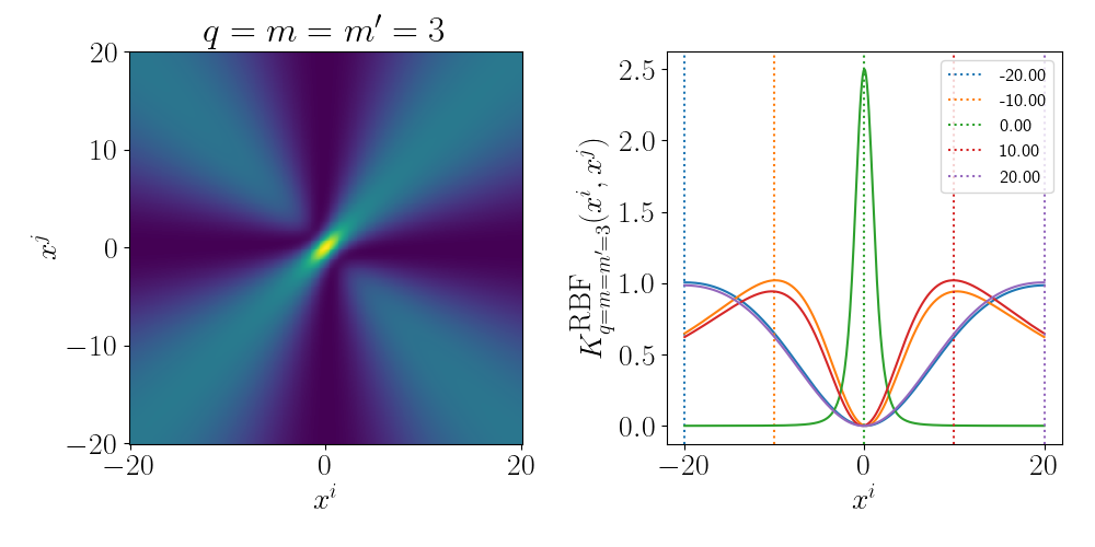
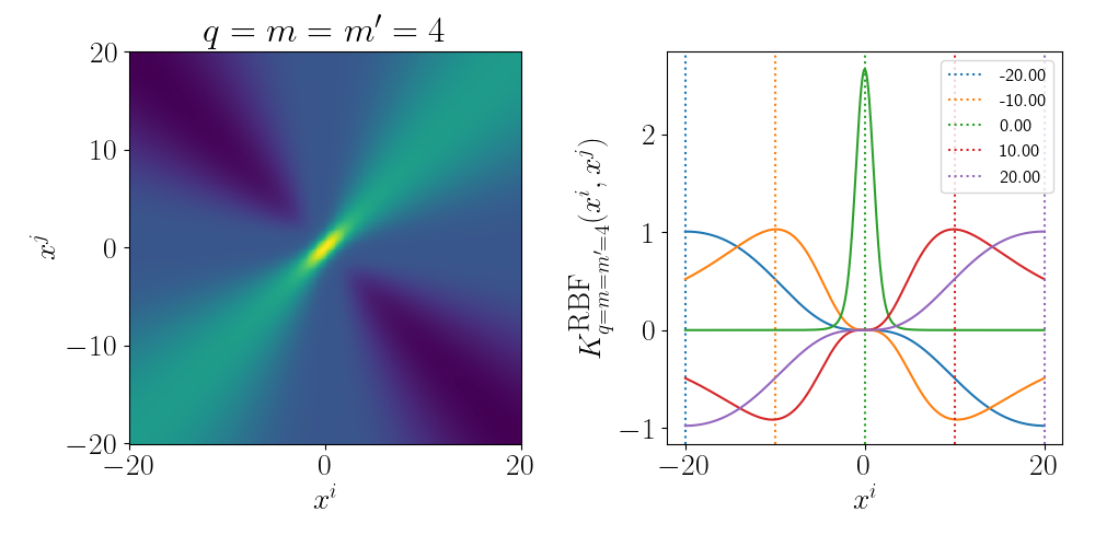
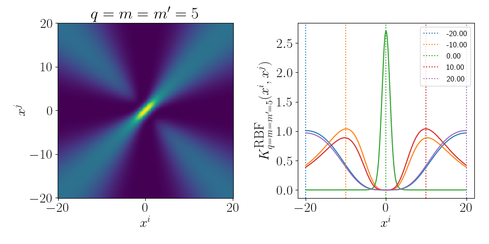
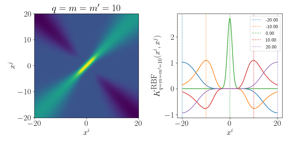
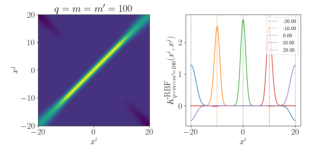
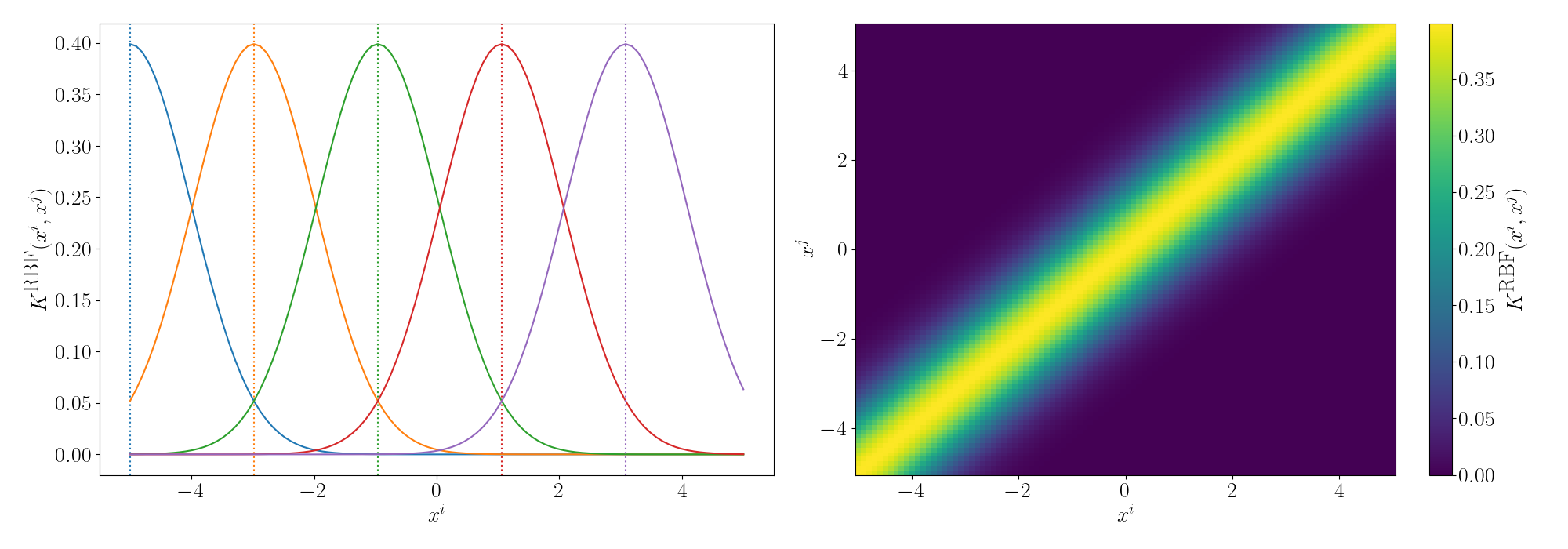
Essentially as stated above, the inner product/kernel function value is large when the variables are of a similar value.

There are a bunch more kernels to model different behaviours including the periodic kernel and Matern kernel, and you can combine them to model different behaviours! You can play around with some different kernels here. It’s a Gaussian Process interactive website that you can just think of it as something that will plot the forms of equations/relationships between coordinates that the kernels imply. I’ll demonstrate some more through the following examples.

Awesome Kernel-Based Methods

Kernel Discriminatory Analysis (KDA II)

Resources

• Kernel Fisher discriminant analysis
• Manifold hypothesis

The Gist

So, apply the kernel trick to Fisher Discriminant Analysis yields us Kernel Fisher Discriminant Analysis or KDA for short. Let’s first have a look at the last example I gave for the support vector model section.

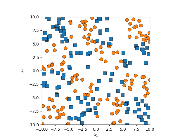
There isn’t an easy way to see what polynomial kernel would be able to distinguish between the two groups here. So let’s just examine the behaviour as we increase the degree of the polynomial kernel.

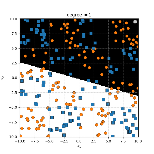
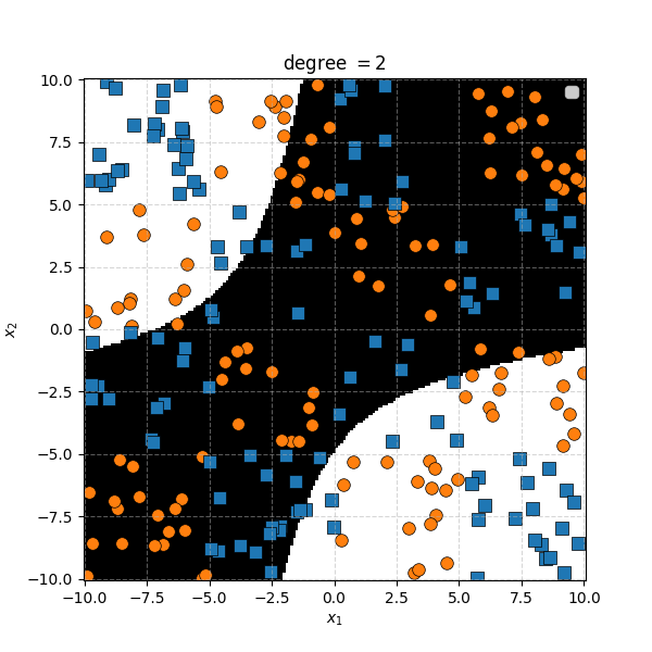
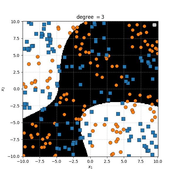
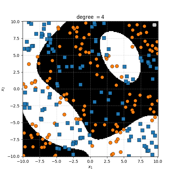
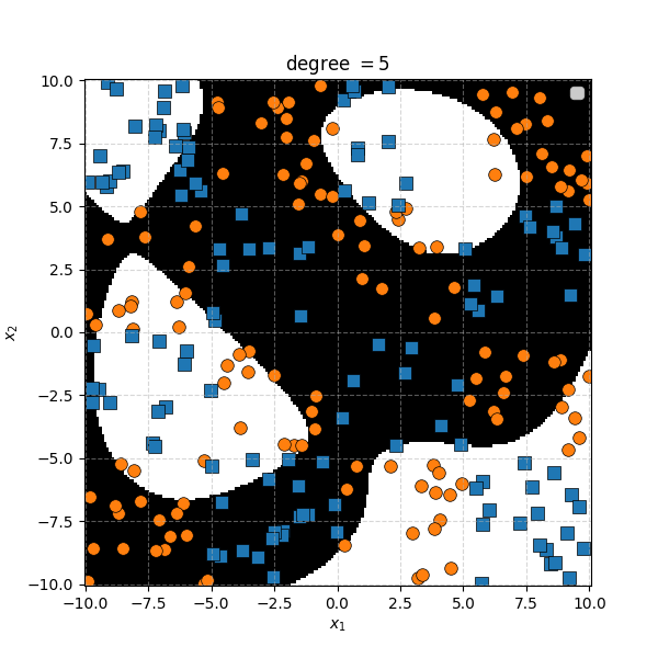
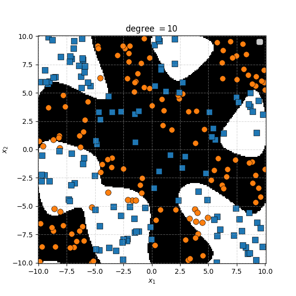
So the degree 1 polynomial kernel correspond to the linear separation boundary and degree 2 you can intuit is the same as the quadratic decision boundary. As we increase the degree of the kernel we can extract more fine tuned decision boundaries but it also becomes more susceptible to overfitting and noise. And we get to do all this without actually having to store or calculate within the project polynomial spaces!

In this case we can just immediately tell that the data is formed into blocks of groups, so it might be better to apply the RBF kernel that allows us to encode behaviour based on the distances between the points. Scaling the \(\gamma\) or equvialently the \(\sigma\) of the kernel changes the length scale that we presume the data is following. Let’s also have a look at these and see the impact on the decision boundaries that the KDA implies.

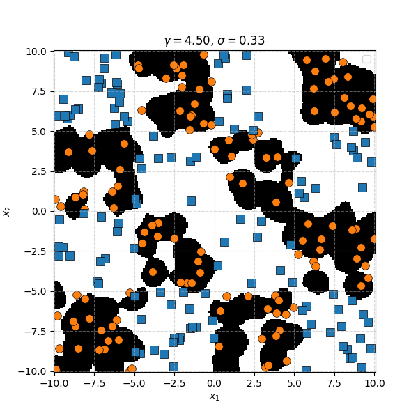
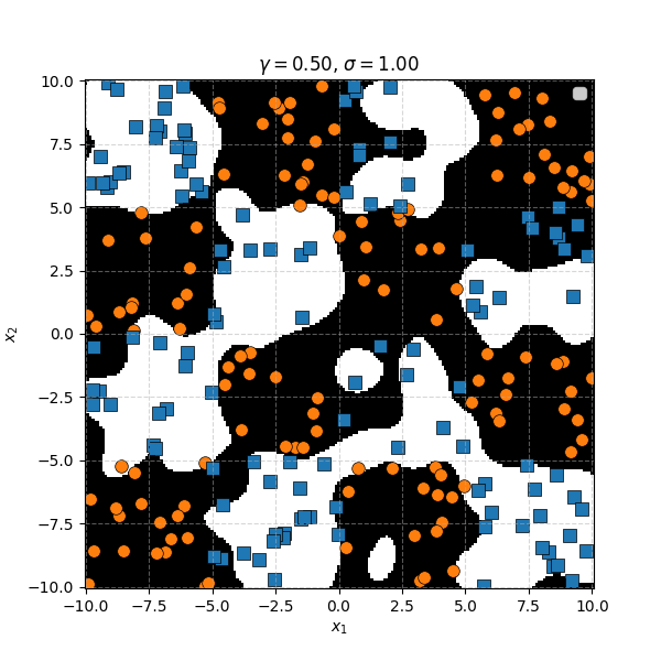
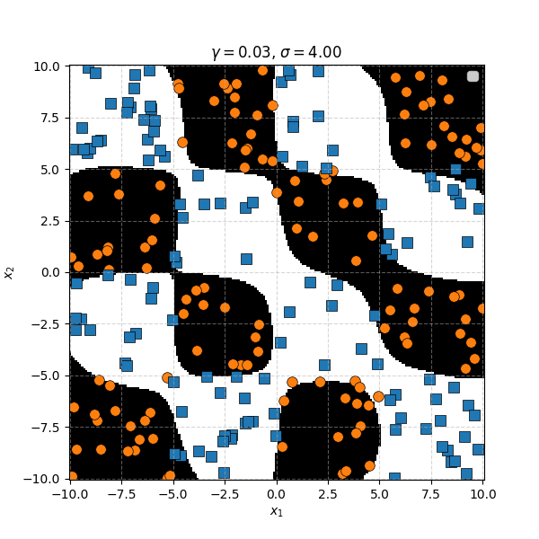
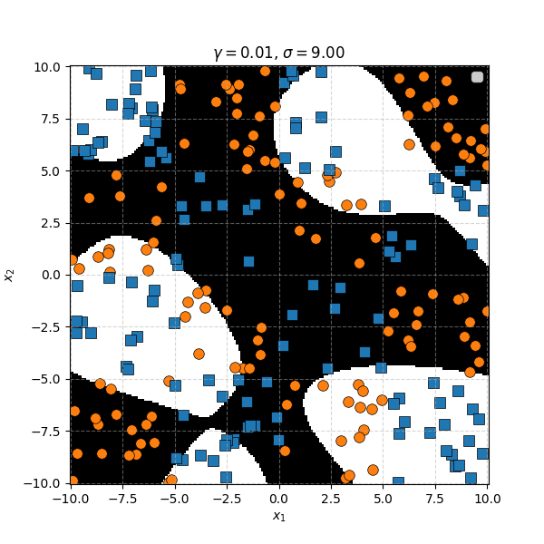
We can see that for smaller values of \(\sigma\) we can capture features on a smaller scale, but again, we become more susceptible to noise. While for larger length scales we can capture larger scale features or behaviours. In this case I would say that a length scale of 4 worked the best, which closely matches the checkboard pattern that I use to generate the samples which you can see below.

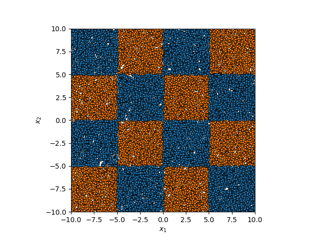
Here’s the code that used to do the KDA, all that it required was using the Gram matrix, K, and using that in place of the explicit dot products in the original section.

Support Vector Machines (SVM II)

Resources

• Manifold hypothesis
• Support Vector Machine - Wikipedia
  • Only once did I get to this section did I realise how unoriginal I am sometimes. My support vector model plot is almost exactly the same as the Linear SVM plot on this page
• CS229 Lecture notes - Support Vector Machines

The Gist

The inclusion of the kernel is what turns a basic support vector model into the widely used support vector machine. Remember from the previous section on the topic that our loss was as follows,

To make this ‘kernel-ized’ we can imagine the projection operation into the higher dimensional spaces we were doing as some sort of transformation, \(T\), and chuck that in.

We then can replace that dot product by the kernel of our choice, \(K(\vec{x}_i, \vec{x}_j)\),

Then boom! We have a kernel-based method! Now let’s see how much better/worse the support vector machine setup does compared to the KDA setup on the checkerboard example.

Instead of writing my own code this time I’m just using `sklearn.svm.SVC’ which is a support vector machine classifier which I modelled the inputs on my custom class above on. First we can look at the polynomial kernels.

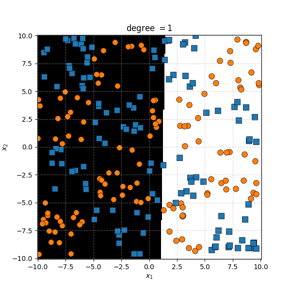
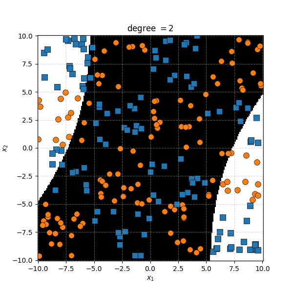
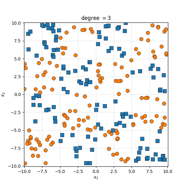
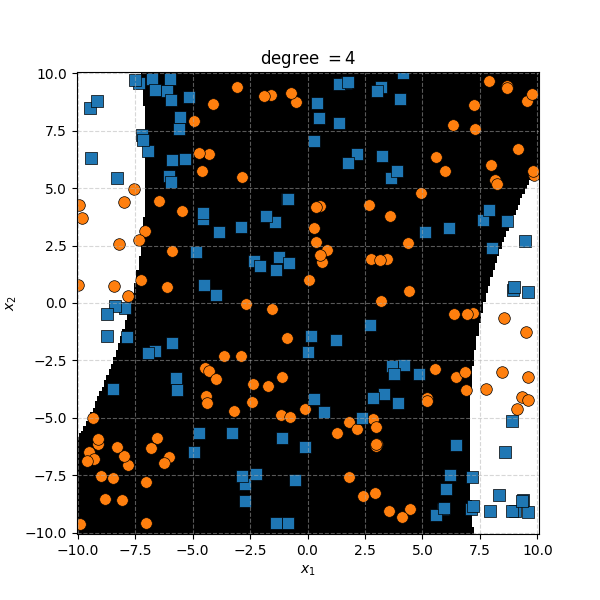
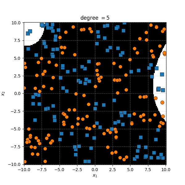
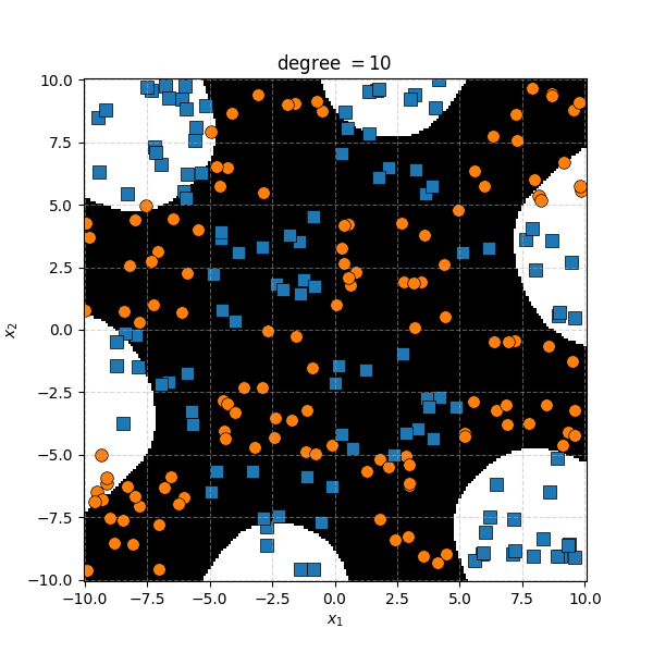
It seems the support vector machine is doing notably worse. However it generally isn’t fitting random noise variations like the KDA approach did. Likely because the data is so noisy that it can’t create reasonable margins very well. And then the RBF kernels.

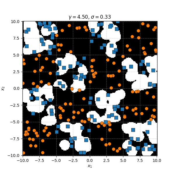
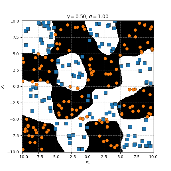
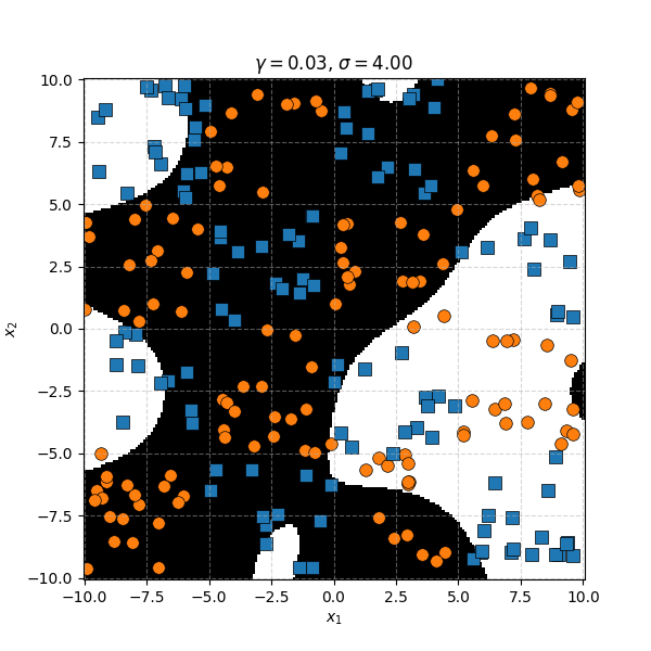
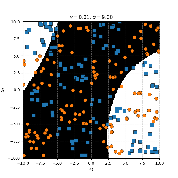
Similar to before, for this specific dataset the SVM isn’t doing as well. However, it’s interesting to note that in the case of the very small length scale it does pretty well. Eespecially if you compare it to the equivalent KDA plot that seems to be not really picking up any overall structure while the SVM seems to be doing so.

And quick side note, using the above class you can extract the support vectors being used to make the decision boundaries. In the cases above however it turns out to be almost every single point so I didn’t see the point either.

Kernel Ridge Regression (KRR II)

Resources

• Kernel ridge Regression - Max Welling
• Kernel method
• Kernel regression - Wikipedia
  • Only useful as far as to know that it isn’t the same as Kernel Ridge Regression
• Kernel Methods and SVMs - Justin Domke
• Kernel Ridge Regression - Cynthia Rudin
  • Is much simpler than what I have, but I didn’t like a substitution that they make at the beginning without a robust explanation. I basically follow what they do after I express \(\vec{\alpha}\) in terms of \(\vec{\beta}\)
• Comparison of kernel ridge and Gaussian process regression - scikit learn documentation

The Gist

Similar how we transition from linear support vector machines to general support vector machines we can generalise ridge regression but reducing the problem down to just involve dot products between the variables that we wish to project into the higher dimensional feature space.

What we can do is note that the lost function we constructed,

likely won’t actually be able to go to exactly 0, but the optimisation will be done when we reach a local minima with respect to \(\vec{\alpha}\). Hence, taking a derivative of the above and setting it to \(\vec{0}\) we find,

Noting here for clarity that \((Y_i - X_i \vec{\alpha})\) is a scalar and \(X_i \vec{\alpha} = \vec{\alpha}^T X_i^T\) (scalar) with \(P\) being the dimensionality of \(X_i\).

Utilising an identity equivalent Woodbury matrix identity called the push-through identity, with \(U = [m\times n]\) and \(V = [n\times m]\)

we can then move some of this around with \(N\) being the number of observations/datapoints.

Huzzah! \(X X^T\) is just the Gram matrix! If we look at the \(ij^{th}\) entry then it is \((X X^T)_{ij} = X_i^T X_j\). We can see that the terms on the right are all very calculatable with kernels, but the \(X^T\) hanging around out the front is a little weird. Let’s replace the thing that we can calculate efficiently with just \(\vec{\beta}\) of size \([N\times 1]\) such that,

If we plug this into our loss we find something really nice,

There it is again! Plopping in the Gram matrix for \(X X^T\).

So we can efficiently calculate our loss and project our data onto \(\vec{\alpha}\) implicitly (unless \(N\) is large, in which case inverting \(K + \lambda I\) ain’t gonna be easy). Except we don’t really need to optimise now because we already have the solution for a given \(X\) and \(Y\) by projecting any data implicitly by the \(K \vec{\beta}\) term or for a single observed datapoint \(x_*\), \(\sum_i x_*^T X \vec{\beta} = \sum_i k(x_*, x_i) \vec{\beta}\).

Now that we know that we can do it. Look at the problems from the previous section again. First the basketball data, let’s have a look at some fits for the polynomial kernels and RBF kernels.

First the fits with the polynomial kernel.

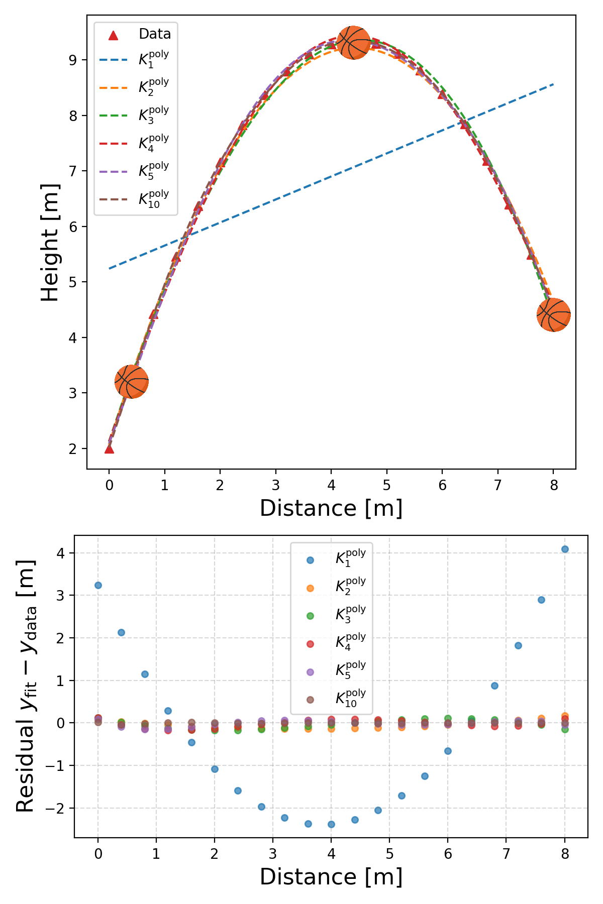
Basically works out to the more the better! And then the RBF kernel.

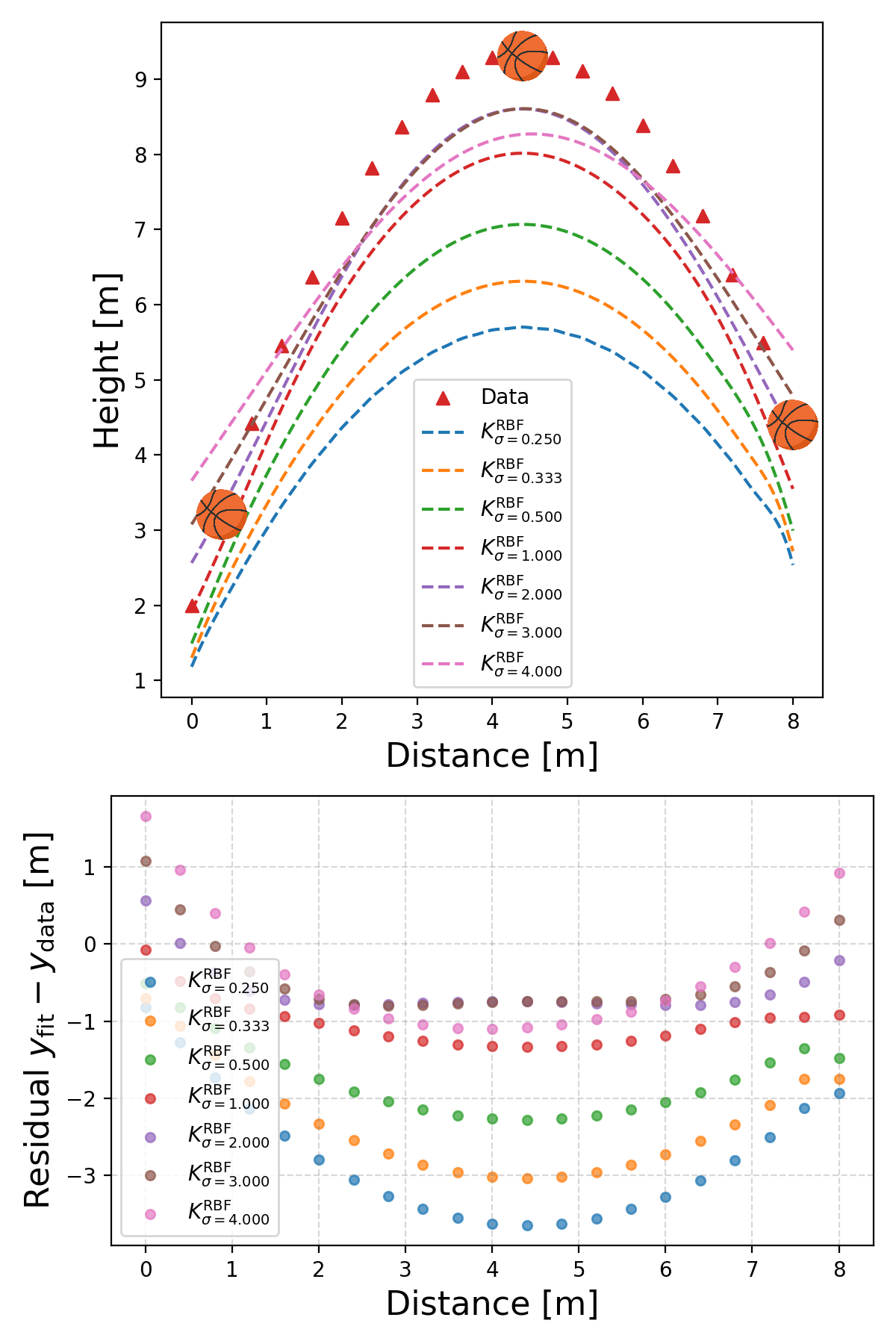
Not as good … basically this is a demonstration that different kernels are suited for different problems. There isn’t a single ‘best’ kernel. For example with the sunspot data.

We obviously have periodic components with non-negative data.

For the periodicity we can use the ExpSinSquared or simply periodic kernel. Functionally what the kernel looks like is the following,

where \(l\) is the length scale again and \(p\) is the period of the kernel. It’s pretty obvious how the periodicity works here, you have a \(\pi\) periodic kernel, you get \(\pi\) periodic functional representations. What’s not immediately obvious, or at least it wasn’t to me, was how the length scale comes into play.

Looks look at some periodic kernel pseudo-Gram matrices for different length scales.

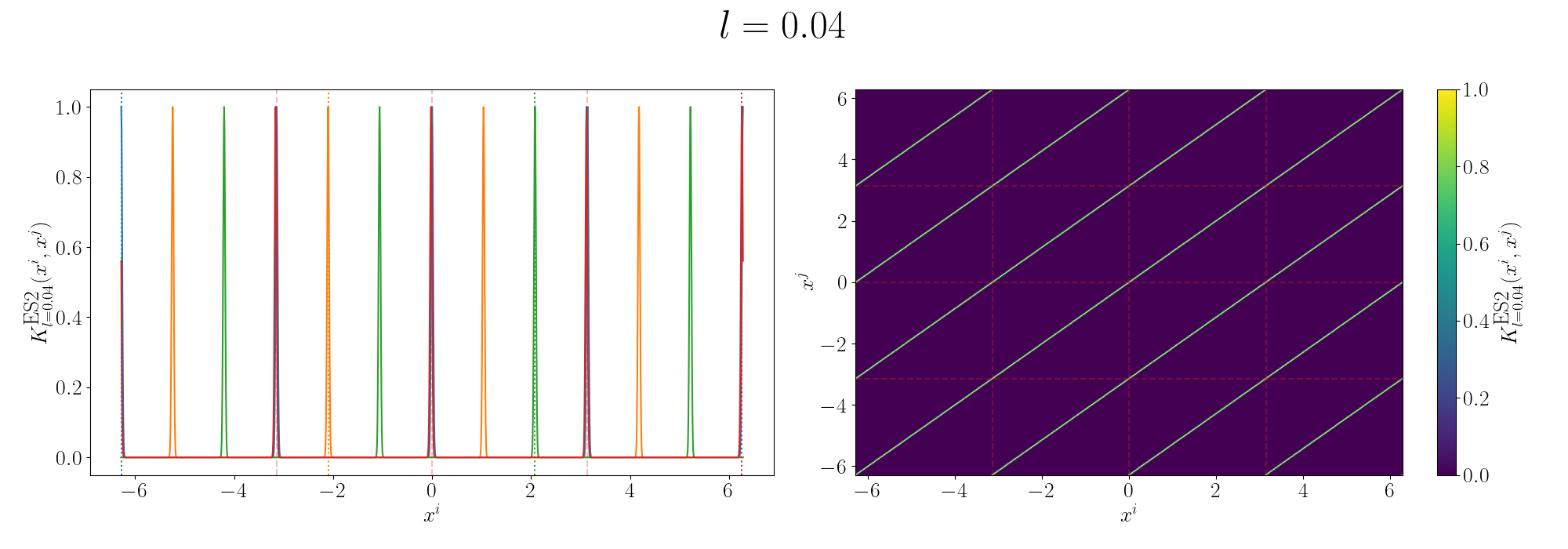
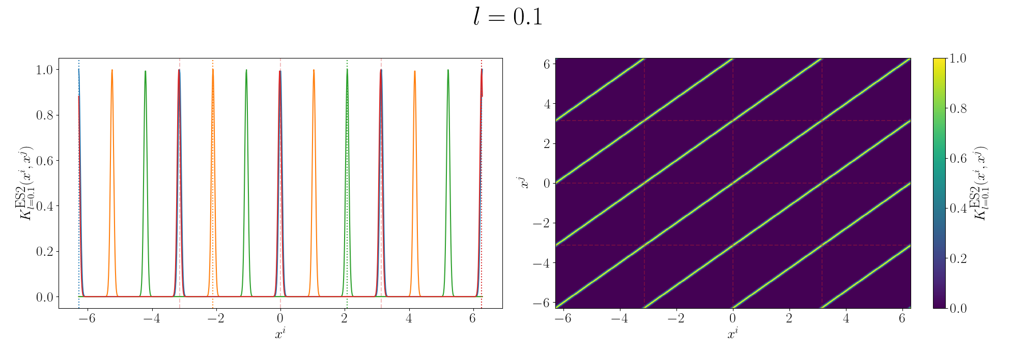
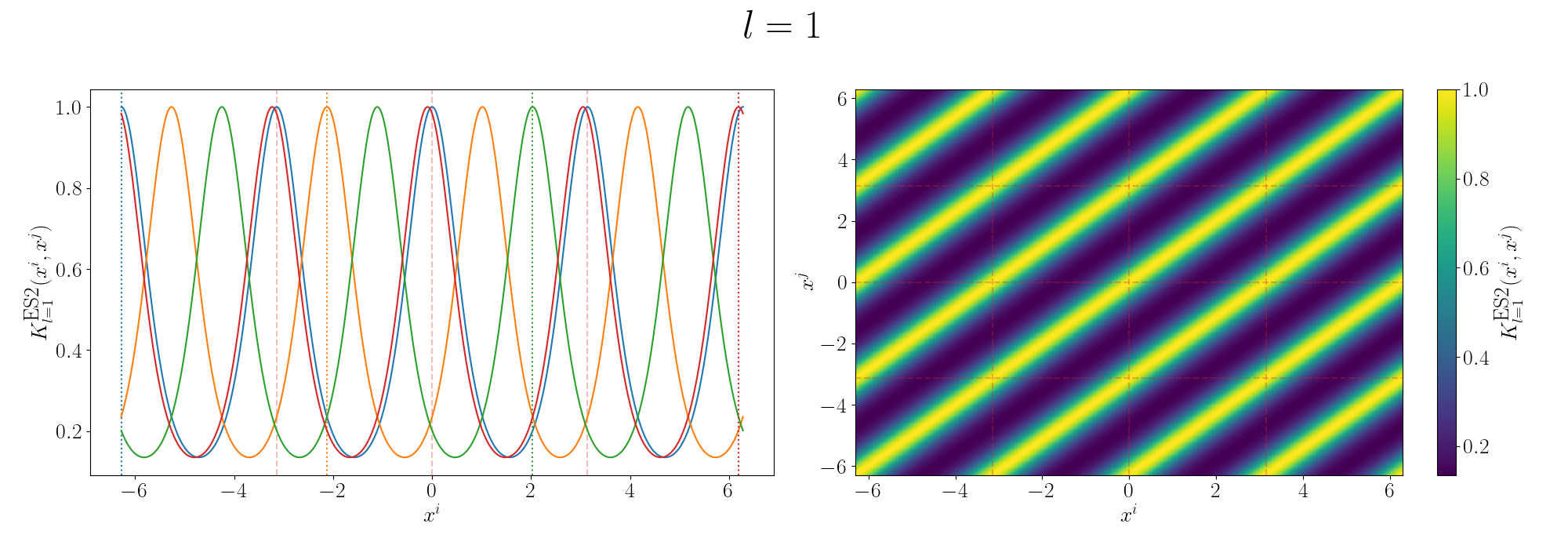
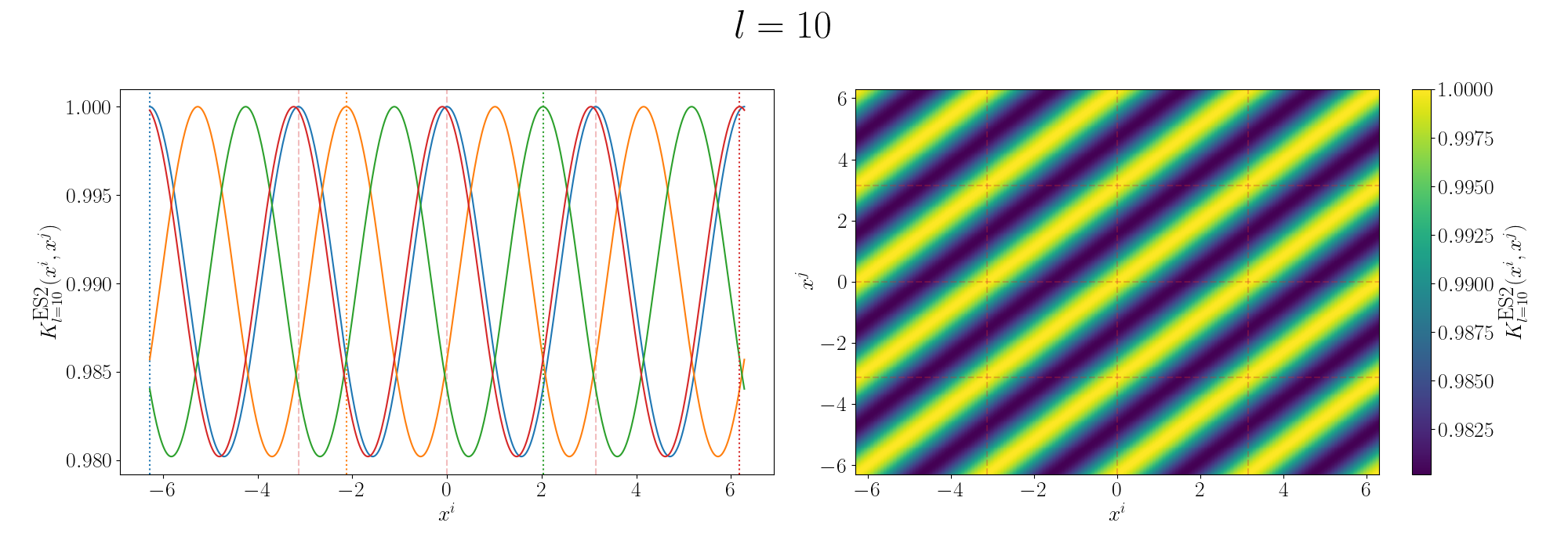
Remembering that these plots are showing the inner products between our inputs we can see the obvious periodicity, we except values that are some integer multiple of \(\pi\) apart from each other to be related. The length scale seems to be how hard of a relationship we want to expect/how much we are fine with deviating away from exact periodicity.

• For large values of the length scale we can model very smooth behaviour where nearby values to the exact integer distances are still meaningfully related.
• For small values of the length scale we model very rough or rapidly changing behaviour, with only values extremely close to the exact integer distances giving non-zero values of the inner product.

And this isn’t just the case for the periodic kernel, the length scale pretty much always behaves this way. Large = smooth and small = rough/rapidly changing or for behaviours that deviate from pure sinusoidal components.

Now, going back to the sunspot data. I couldn’t figure out a good way that wasn’t really ad-hoc for or even gave significantly better results ensuring the non-negativity so we’ll focus on the periodicity. We can first identify that the data isn’t a pure sinusoid. No duh. And that there are likely more than I frequency making up the data.

The remaining question is then how do we handle the multiple frequencies/periodicities? Well if we want to combine the behaviour of multiple kernels (in this case multiple periodic kernels) it’s actually pretty simple. To combine different kernels we can simply add or multiple the function outputs together. In this case I’m going to multiply them together as I think the relationship in the data is something like a periodic signal modulated by some envelope/another periodic component.

For now let’s say that the kernels have the same length scale, and for simplicity we’ll set it to one. Then the derived kernel is something like,

Let’s look again at some examples of the Gram matrix.

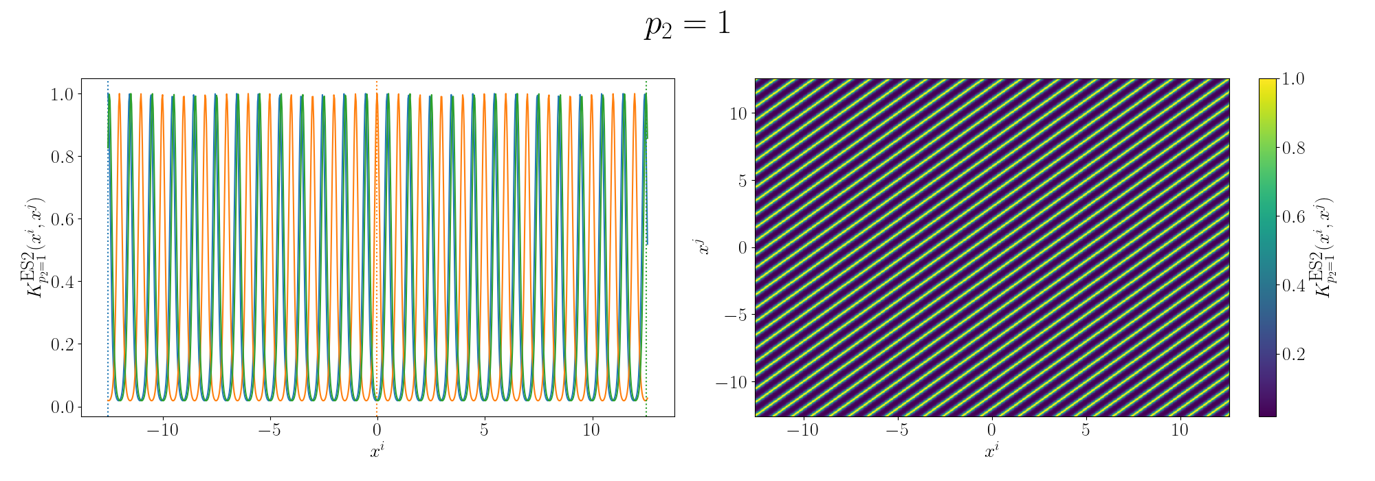
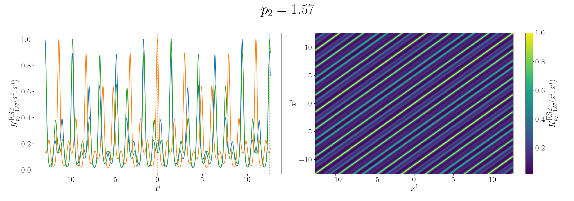
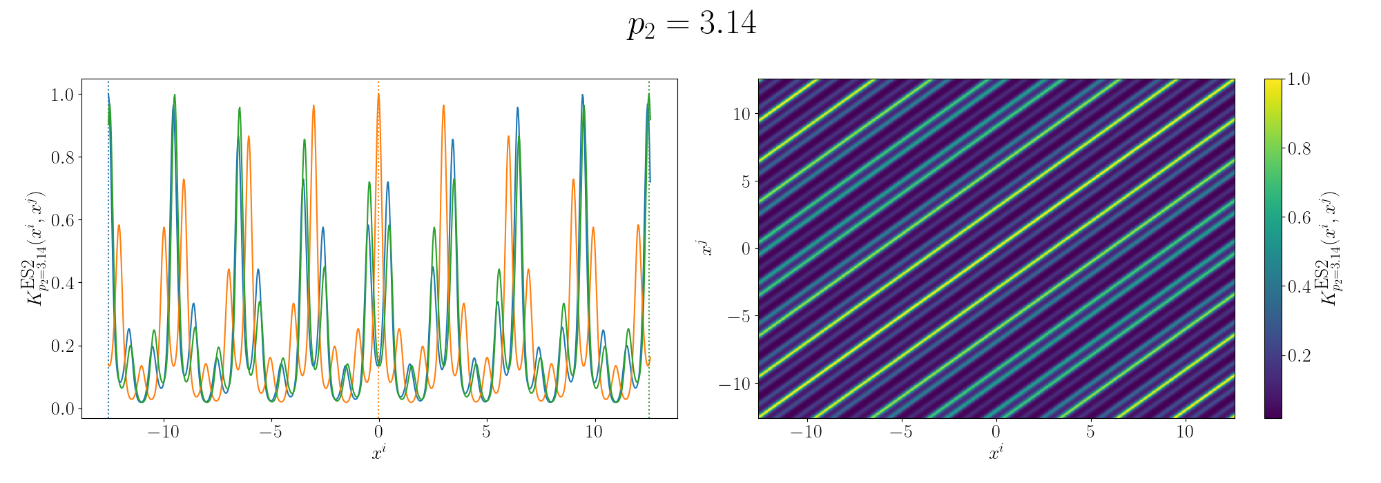
So you can see that we kind of see the functional form of the behaviour we’re expecting⁶. We can also look at the same graphs for if we added the kernels instead.

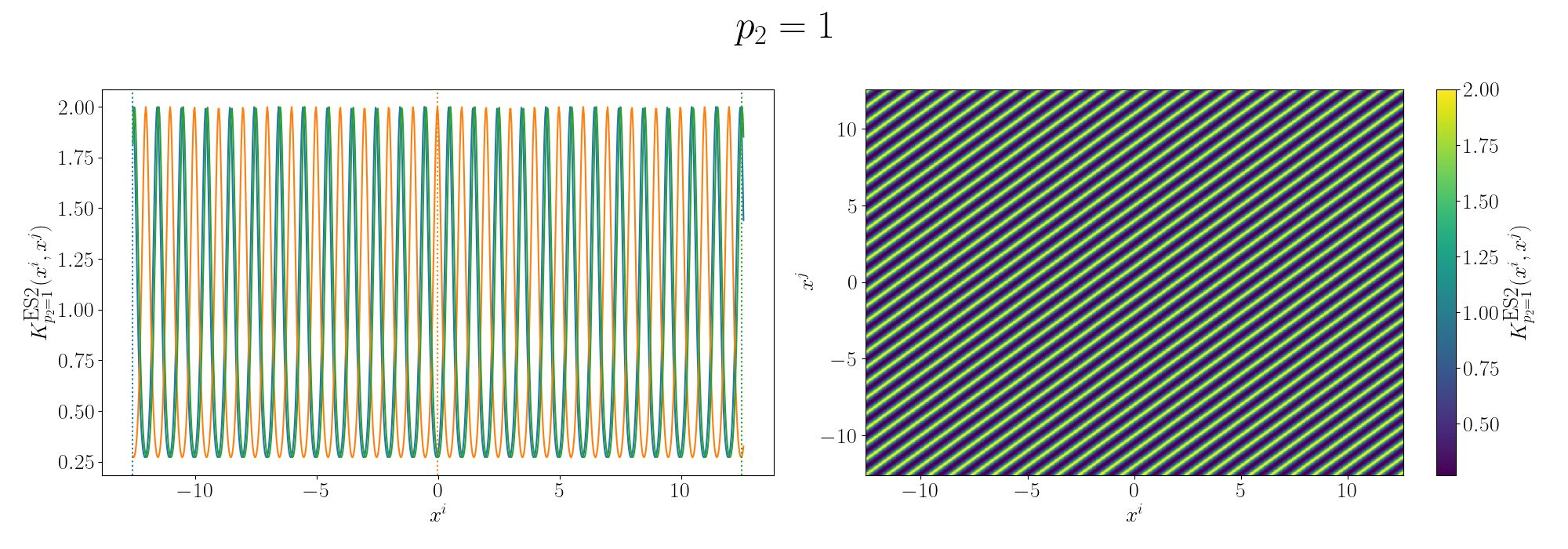
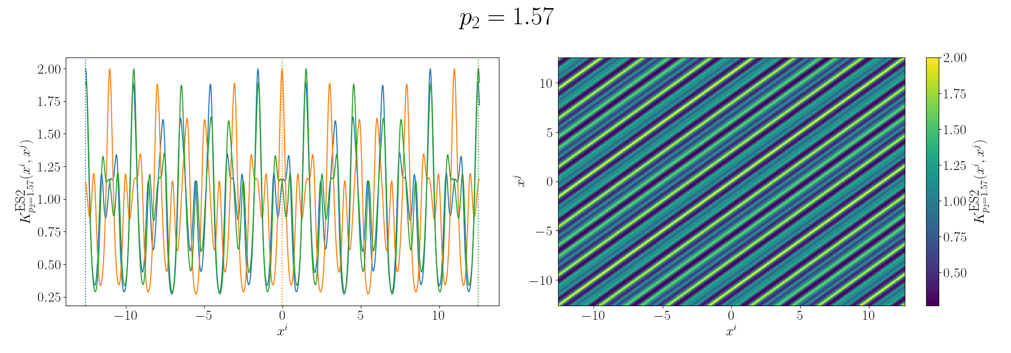
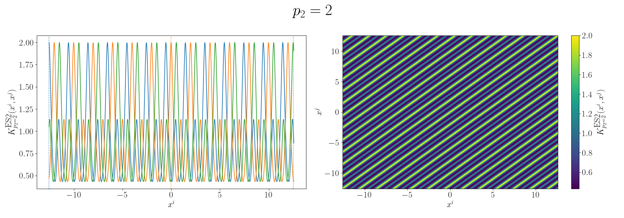
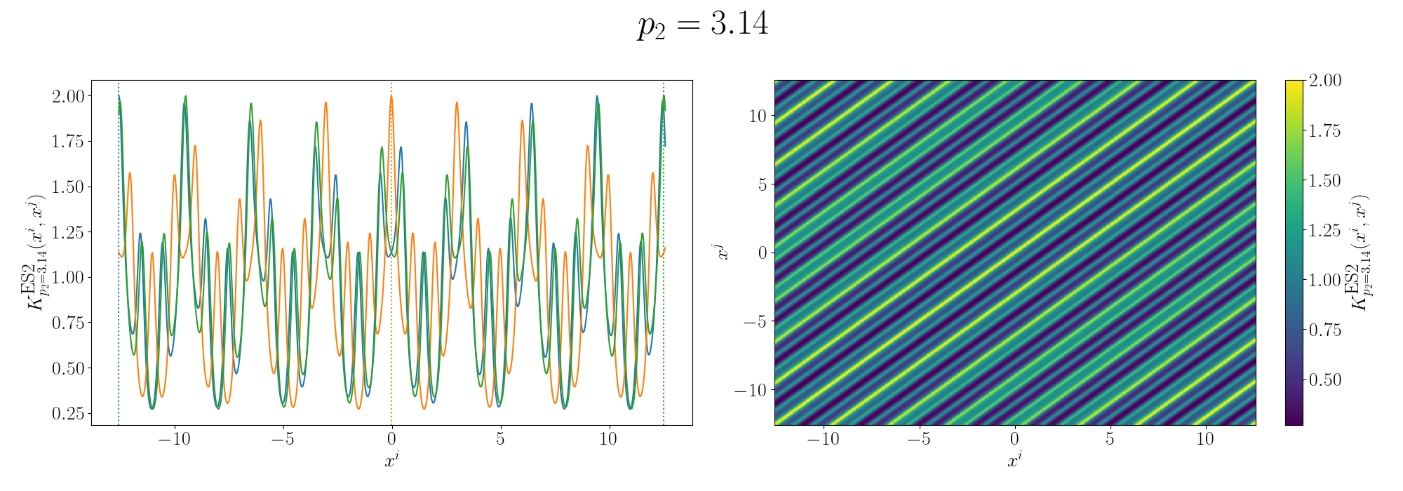
So the additive version generally looks like you’ve added two sinusoidal functions together and broadly kind seems to relate the points in a similar looking way to the sunspot data. I’ll go into more details in the Gallery of Kernels section.

But at the end of the day, I was testing out both of them, and the compound/multiplied kernels seemed to do the best.

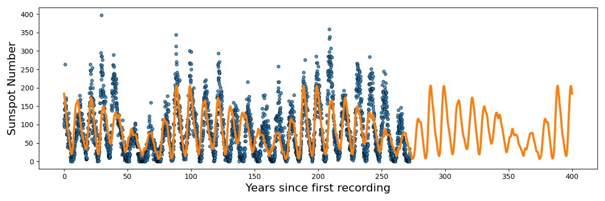
Here’s the code to reproduce the above.

from sklearn.gaussian_process.kernels import ExpSineSquared

sunspot_data = pandas.read_csv("sunspots/Sunspots.csv")
sunspot_data['Date'] = pandas.to_datetime(sunspot_data['Date'])


first_record = sunspot_data['Date'].min()

# 2. Calculate the difference (timedelta)
time_difference = sunspot_data['Date'] - first_record

# 3. Convert the timedelta to total days (as a float)
# .dt.total_seconds() returns the difference in seconds
# / (60 * 60 * 24) converts seconds to days

days_since_first = time_difference.dt.total_seconds() / (365 * 60 * 60 * 24)

sunspot_X = days_since_first
sunspot_design = np.array([np.ones_like(days_since_first), days_since_first]).T
sunspot_Y = sunspot_data['Monthly Mean Total Sunspot Number']



kernel = (ExpSineSquared(5.0, 10.0, periodicity_bounds=(1e-2, 1e3)) 
    * ExpSineSquared(5.0, 100.0, periodicity_bounds=(1e-2, 1e3)) \
    # * ExpSineSquared(60.0, 60.0, periodicity_bounds=(1e-2, 1e3)) \
    )
regression_cls = KernelRidge(alpha=1e-8, kernel=kernel)

regression_cls.fit(sunspot_design, sunspot_Y)

num_times = 2000
test_sunspot_X = np.linspace(0, 400, num_times)
test_sunspot_design = np.array([np.ones(num_times), test_sunspot_X]).T


sunspot_Y_fit = regression_cls.predict(test_sunspot_design)

plt.figure(figsize=(12, 4))
plt.scatter(sunspot_X, sunspot_Y, s=20, lw=0.5, edgecolor='k', color='tab:blue', label='Data', alpha=0.8)
plt.plot(test_sunspot_X, sunspot_Y_fit, color='tab:orange', label='Kernel Ridge Prediction', lw=3.0)
plt.xlabel("Years since first recording", size=16)
plt.ylabel("Sunspot Number", size=16)
plt.tight_layout()
plt.savefig("KRidge_Figures/sunspot_data_with_kernel_ridge_fit.png")

plt.show()

And one just keeps multiplying with more and more periodic kernels you can get something that looks like this. At this point though it’s likely overfitting.

Kernel Principle Component Analysis (Kernel PCA II)

Resources

• Manifold hypothesis
• Kernel Principal Component Analysis - Bernhard Scholkopf (pdf link)
• What Are the Advantages of Kernel PCA Over Standard PCA? - Enes Zvornicanin
• Dimensionality reduction. PCA. Kernel PCA - COMP-652 and ECSE-608
• ML | Face Recognition Using Eigenfaces (PCA Algorithm) - pawangfg

The Gist

No I’m going to come right out of the gate with the fact that most of the time Kernel PCA or KPCA is not going to be useful to you in the same way that PCA is. Arguably the main benefit of PCA is that you are able to generate a very interpretable combination of your parameters that nicely explains most of the variation in your data. It does however allow separation of data in a similar way if that’s your game.

For example, stealing an example right from the scikit-learn page on KPCA.

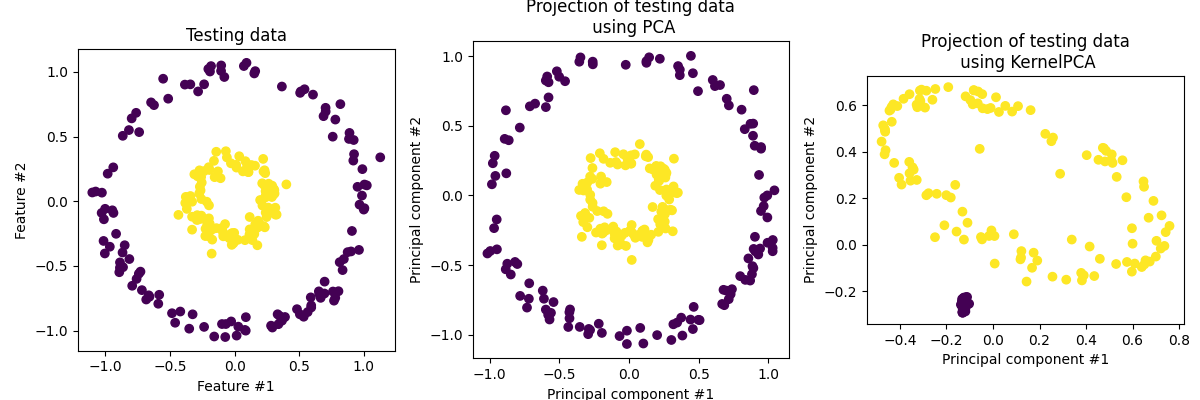
The interpretability aspect in traditional PCA is because it presumes a linear relationship so any combination comes out to be similar to a weighted representation of how much each component contributes to the variation. It’s more often used as a dimensionality reduction technique than standard PCA particularly within the machine learning community. You can interpret the component coefficients of the as a representation of the data and use that as a smaller input to feed into a neural network or as a smaller latent space to learn key features of the data like an autoencoder for example. (stealing the example from the same page).

But I’m getting ahead of myself, let’s just see how it works first. As a reminder what we did was construct a covariance matrix,

and then performed a eigen value or singular value decomposition to find the eigenvectors along which the variation in the data is maximised (particularly the first eigenvector),

and we could use those eigen vectors, e.g. \(u_j\), and project our data on to them using a dot product \(u_j^T \vec{x_i}\). The key insight here is that if we describe the covariance matrix as the following sum of outer products,

where \(\Phi(x_i)\) denote the vectors in the projected feature space, then as any eigen vector can by definition be described as \(\lambda_j v = S v_j\) if we place this in the equation immediately above then we find,

(chucking the \(\lambda_j\) at the end and absorbing the \(1/n\) to make the following math nicer). This means than any eigenvector in the feature space can be described as a linear combination of the data points in this space.

No we can’t calculate the actual covariance matrix in the feature space as it would quickly get to big (and for RBF infinite!). But going back to the original PCA, what we really wanted was to project the data on to the PCA components and record the given result as value in this component dimension. So if we imagine that we wanted to project one of our data points \(\Phi(x_m)\) onto a given component in feature space it would look like the following.

Dot product with the given component.

That shows that we can represent the dot product as a linear combination of the kernel values. But then what’s \(\alpha_{ij}\)? For this we’re going to chuck our \(v_j\) back into the eigenvalue/vector equation.

Then we’re going to do something sneaky and multiply both sides by some arbitrary point projection of our data⁷, \(\Phi(x_q)\), and substituing our solution for \(v_j\) again on the LHS,

Hopefully you can see that in the LHS sum between the kernel and \(\vec{\alpha_j} = \{\alpha_{1j}, \alpha_{2j}, ..., \alpha_{nj}\}\) is a matrix product, more specifically a dot product (!). And the right hand side has a couple dot products, that we can represent as the following where \(K_{qp} = k(x_q, x_p)\).

Assuming that \(K\) has an inverse then we get a new eigenvalue problem,

In essence, instead of taking the eigenvalues and eigenvectors of the covariance matrix we take the eigenvalues and eigenvectors of the gram matrix!

Now let’s go back to the following dataset.

First let’s actually see how the standard PCA performs on the data.

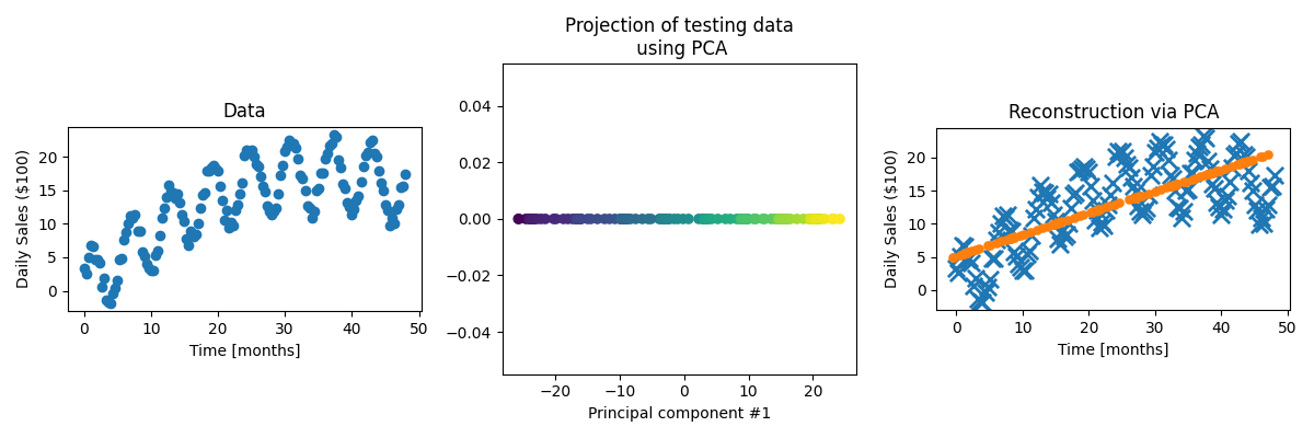
For the data, it’s obviously done the best it can when presuming a linear relationship but is clearly missing some key information.

Now applying kernel PCA, we’re definitely seeing a periodic behaviour with some periodicity on the scale of ~6 months? And I’ll just guess a length scale around 5. Let’s try just the periodic kernel and see how it does.

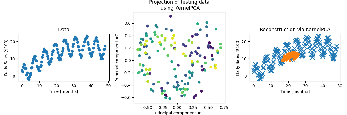
Not very good! The projection of the data into the components is Which is good! Because there’s obviously some polynomial (quadratic I would guess) behaviour so it’d be weird if we got everything to work with just the periodic kernel. Let’s multiply the periodic and polynormial degree 2 kernels together and see how we do. The data in the projected space looks like…

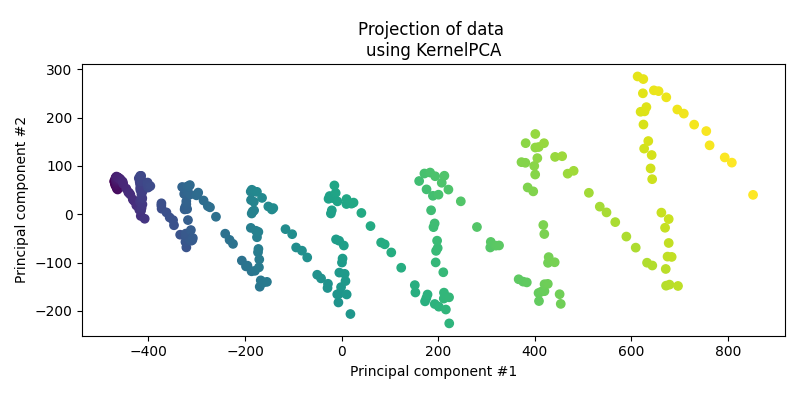
We can see that one component seems to be broadly tracking time and the other the amplitude which is a good sign. Let’s see how well we can reconstruct the data (extra easy as the testing data is also the training data).

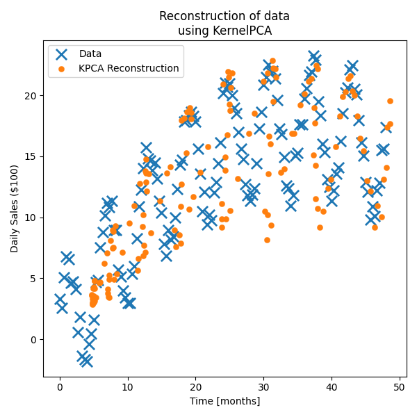
Much better! Still not fantastic if we’re being honest, but it’s obviously picking up some of the periodic and quadratic behaviour. Now let’s see how much information using 1 component KPCA retains with the same amount of training data but

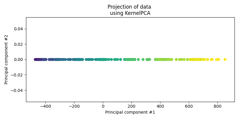
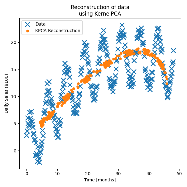
Cool! We’ve lost the periodicity but we’ve actually kinda got the trend better than for 2 components?

Gaussian Processes

Resources

• A Practical Guide to Gaussian Processes
• Interactive Gaussian Process Visualization
• Gaussian process regression demo
• Gaussian Processes for Machine Learning
• 2023-01-09 PRML - From Bayesian Linear Regression to Gaussian processes - Stefan Harmeling
• A Visual Exploration of Gaussian Processes - distill

The Gist

Gaussian processes is where I want to finish this post. It and KPCA were the main topics that I wanted to cover. But unlike KPCA, Gaussian processes to me were much harder to initially get a grasp on. However, if you’ve followed me up until this point, you’ve already done the hard work, because I’ve secretly already gone through the most of the main ideas of Gaussian processes through the sections on Kernel Ridge Regression. In fact one can (and one will) show that Kernel Ridge Regression is the mean result of the Gaussian process result.

(For those already ahead of me I’m quite following the weight-space explanation here)

So back-tracking a little through the section on standard Ridge Regression, we were interested in fitting a straight line to data, encapsulated in the likelihood.

or maybe more formulaically,

We then said that \(\vec{\alpha} \sim \tau \mathcal{N}(\vec{0}, \vec{1})\) and finally arrived at the expression for the posterior to be proportional to,

Then minimisation of the negative log-posterior ensued. With Kernel Ridge Regression replacing any dot products with the kernel function so that we could implicitly project our data into higher dimensional feature spaces and do linear regression there. Thus allowing us to do non-linear regression in the original data space.

There are two ways that we will deviate from the above:

1. We will allow for a more general prior on \(\vec{\alpha}\) –> \(\vec{\alpha} \sim \mathcal{N}(\vec{0}, \Sigma_p)\). Where \(p\) denotes the number of parameters or simply the length of \(\vec{\alpha}\).
2. We will care about uncertainties.

And that’s it, after that you get Gaussian processes (and the first one isn’t even really unique to Gaussian processes, it’s just generally done more often with them). Doing the first part just means replacing the prior in the posterior expression that we made above. If you’re happy with this explanation, and don’t care about the specifics on the math, then skip to the next subsection.

Then through the \({\color{red}\text{m}}{\color{purple}\text{a}}{\color{blue}\text{g}}{\color{green}\text{i}}{\color{orange}\text{c}}\) \({\color{red}\text{o}}{\color{purple}\text{f}}\) \({\color{green}\text{g}}{\color{orange}\text{a}}{\color{red}\text{u}}{\color{purple}\text{s}}{\color{blue}\text{s}}{\color{green}\text{i}}{\color{orange}\text{a}}{\color{red}\text{n}}{\color{purple}\text{s}}\) we can combine the two normal distributions in the following way.

With,

which is just what we found for \(\vec{\alpha}\) previously⁸ i.e. that our result from Kernel Ridge Regression was the mean for the Gaussian process result. But now, instead of using the push-through identity we use the full Woodbury matrix identity.

With no relationship between the variables used above,

Which we can use to rearrange \(\hat{\vec{\alpha}}\) in a similar way that we did before for \(\vec{\alpha}\) in the Kernel Ridge Regression section with,

Now redefining what we represent as the inner product (now a weighted dot/inner product) as,

and thus,

Moving on with this new definition we replace the relevant terms,

Now we’re going to do something sneaky and replace \(I\) with \((K + \sigma^2 I)^{-1} (K + \sigma^2 I)\).

This is basically in the same form as before except \(\Sigma_p\) isn’t assumed to be a constant term multiplied by the identity matrix. So we continue on with the exact same thinking that now we have our solution, let’s project some input data, which when in the infinite dimensional feature space I will refer to as \(\phi(x_*)\) for a second, putting it into an approximate value for output data variable \(y_*\).

defining \(\phi(x_*)^T \Sigma_p X^T = k(x_*, X)\),

With this last term being equivalent to the projection that we got in the kernel ridge regression. i.e. We’ve just slightly generalise our kernel ridge regression result.

If we want something to sample from and get uncertainties for, we need a probability density. Starting over from here,

This encodes the probabilities (up to a constant multiplier) on our parameters \(\vec{\alpha}\), which may be infinite dimensional so isn’t the most handy in practice. What we would want, is uncertainties on our fit, i.e. if we look at a given input \(x_*\) and output \(y_*\) \(p(y_*\vert x_*, \vec{\alpha}, Y, X)\). But then we have the dependency on \(\vec{\alpha}\) still 😢.

What we’re going to do is remove the explicit dependence on \(\vec{\alpha}\) through marginalisation which is basically the reason that I’m using the \(\propto\) instead of \(=\) in the above.

As a refresher, we can describe the conditional probability, \(p(A\vert B)\) via Baye’s theorem,

and if \(A\) and \(B\) are continuous quantities, we know the following by the definition of a probability density,

And with a bit of rearrangement using the fact that \(p(B)\) isn’t dependent on \(A\) then we find,

This process of integrating out the variable \(A\) is called marginalisation and can be thought of as a weighted average of \(p(B\vert A)\) with respect to \(p(A)\)⁹ or a million other ways that I don’t have the time to go through atm. For us, this basically means that if we have some annoying variable \(A\) in our probability density \(p(B\vert A)\) we can integrate it away presuming we have the probability density \(p(A)\)… 🤔

Well, if we wanted \(p(y_* \vert x_*, X, Y)\) we could perform the following marginalisation,

where we have \(p(\vec{\alpha} \vert Y, X)\) up to the multiplicative constant \(p(Y\vert X)\) (with respect to \(\vec{\alpha}\)) and is our original observational likelihood for a single point,

Looking at just the exponent which I’ll denote with \(E\),

Where I’ve replaced some terms with \(A = \sigma^{-2} X^T X + \Sigma_p^{-1}\) to save on some math steps. We combine terms not involving \(\vec{\alpha}\),

This gives us a simplified expression for the exponent,

What we want to do is turn this expression into a gaussian, as we expect that we should get one out due to the “magic of gaussians” and then we’d be able to analytically solve for the integration. So we want something like \(( \vec{\alpha} - \text{const1})^T \cdot \text{const2}^{-1} \cdot ( \vec{\alpha} - \text{const1})^T\) then we’ll be set. Hence, we find,

We can then pull the constants out of the integral, and now the the gaussian in \(\vec{\alpha}\) bit integrates to a constant (the normalization factor \((2\pi)^{D/2}\vert M_*\vert^{-1/2}\)). We are left with the predictive distribution for \(y_*\), which is determined just by the ‘constants’ terms in the exponent we pulled out:

Now we want something that looks like a gaussian again, because gaussians (or more specifically normal distributions) are \({\color{red}\text{m}}{\color{purple}\text{a}}{\color{blue}\text{g}}{\color{green}\text{i}}{\color{orange}\text{c}}{\color{red}\text{a}}{\color{purple}\text{l}}\). So we want to expand this and get it into something like \(( y_* - \text{mean})^T \cdot \text{cov}^{-1} \cdot ( y_* - \text{mean})\). We already known what the constant will be, it’s the mean prediction, which is the projection of our data onto the mean parameter vector, i.e. what we got from the kernel ridge regression part above. Hence, we just need to find the covariance matrix, so we’ll similarly throw out terms that don’t involve \(y_*\) so that we can just complete the square. So then we can skip the math and just look for the \(y_*^T \cdot \text{cov}^{-1} \cdot y_*\) term.

Now we’re going to remember the fact that in this post we will assume \(y_*\) is a scalar so we \(y_*^T = y_*\) and move it around to find that the term just involving \(y_*\) or simply, the covariance \(\Lambda_*\) looks like,

I swear we’re almost done. Now, the term in the brackets represents the inverse variance of our prediction \(y_*\). But it looks similar to the Woodbury Identity once we expand that middle term \(M_*^{-1} = (A + \sigma^{-2} x_*^T x_*)^{-1}\).

Skipping the matrix gymnastics (which involves expanding the inverse and multiplying by the surrounding terms), this collapses to,

So, our predictive distribution is a Gaussian with the mean we found earlier (Kernel Ridge Regression) and a variance that includes both the inherent noise and our model uncertainty:

Where:

• Mean: \(\mu_{pred} = k_*^T (K + \sigma^2 I)^{-1} Y\)
• Variance: \(\Sigma_{pred} = \sigma^2 + x_* A^{-1} x_*^T\)

Or, if we write the variance purely in terms of kernels (where \(k(x_*, x_*) = x_* \Sigma_p x_*^T\)):

And that is the full Gaussian Process result. We have a mean prediction that matches Kernel Ridge Regression, but now we have a variance term/probability density that allows us to sample different values.

Example Cases using Gaussian Processes

So from our math we found that a gaussian process is just straight line regression but in some projected higher dimensional space that is encoded through a kernel function that allows us to calculate the inner products in that space with the following gaussian probability density,

Where:

• Mean: \(\mu_{pred} = k_*^T (K + \sigma^2 I)^{-1} Y\)
• Variance: \(\Sigma_{pred} = \sigma^2 + x_* A^{-1} x_*^T\)

One extra step that is often useful, is that the above is the predictive distribution for a given observation, but we quite often want the fundamental function that the observational noise is added on top of. This slightly simplifies the above to have,

• The Same Mean: \(\mu_{pred} = k_*^T (K + \sigma^2 I)^{-1} Y\)
• A Different Variance: \(\Sigma_{pred} = x_* A^{-1} x_*^T\)

Now, could we code this up ourselves at this point, probably. Will I? No.

To keep the code even simpler again we will use scikit-learn implementation of gaussian processes, but there are a few other packages out there. Some of which Shun Cheung goes through in their blog post on GPs.

We’ll first take some simple data to show an example of how one can perform regression with gaussian processes. Let’s use that oscillating quadratic ice cream data we used for the kernel PCA.

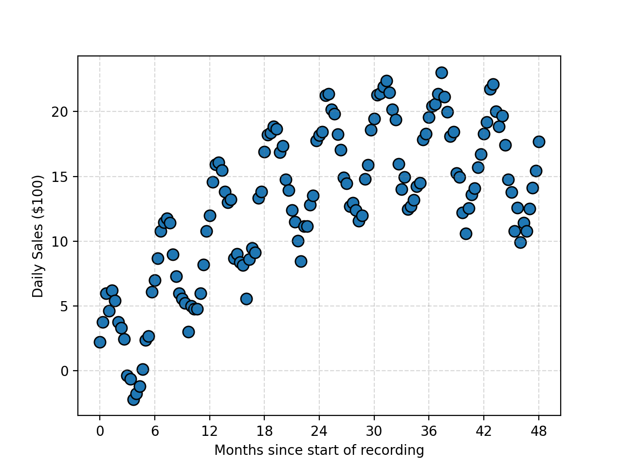
This has three main components that we can make out by eye:

1. A periodic oscillatory component
   • With some periodicity on the order of \(\sim 12\) months
2. Some polynomial component
   • we know it’s degree two but in practice we wouldn’t know.
   • So let’s try degree 4 and add some regularisation such that if the coefficients of the higher order terms aren’t needed they will simply go to 0.
3. Some noise
   • On the order of \(\sim 0.5\)

Hence, our code (including that to generate the data) will look like the following. And I should say there is likely more of just trying stuff out and seeing if it works than I’m letting on.

import numpy as np
from scipy.stats import norm
from matplotlib import pyplot as plt
from sklearn.gaussian_process.kernels import ExpSineSquared, DotProduct, Exponentiation, WhiteKernel, ConstantKernel, PairwiseKernel

########################
### Generating the data
freq = 1

shift = -1

num_years = 4
num_months = num_years * 12
time_months = np.linspace(0, num_months, 3*(num_years * 12) + 1)
ice_cream_data_clean = 5 * np.cos((time_months + shift) * 2 * np.pi * freq/6) + ( 1 * time_months - (0.12 *time_months)**2)

ice_cream_data = ice_cream_data_clean + 0.75*norm().rvs((len(ice_cream_data_clean),))

fake_ICECREAM_X = np.array([time_months, ice_cream_data]).T

#######################################
### Doing gaussian process regression

#######
## Constructing the kernel

# periodic component with unknown contribution, encapsulated in a constant kernel multiplied with a periodic
k_periodic = ConstantKernel(1.0**2) * ExpSineSquared(
    length_scale=1.0,             # Controls the smoothness of the cycle
    periodicity=12.0,             # Fixed at 6 months
    periodicity_bounds=(3, 24),   # Forcing the periodicity to be between 3 and 24 months
)

# polynomial component with unknown contribution, encapsulated in a constant kernel multiplied with a polynomial
k_polynomial = ConstantKernel(1.0**2) * PairwiseKernel(metric='poly', pairwise_kernels_kwargs={'degree':4})

# noise component with assumed noise around 0.5
k_noise = WhiteKernel(noise_level=0.5)

# Adding the components together
kernel_final = k_periodic + k_polynomial + k_noise


# Instantiating the gaussian process object
simple_gaussian_process_1 = GaussianProcessRegressor(
    kernel=kernel_final, 
    n_restarts_optimizer=50, #30,
    alpha=1e-1
)

# Fitting the gaussian process hyperparameters to the data
simple_gaussian_process_1.fit(
    time_months.reshape(-1, 1), 
    ice_cream_data.reshape(-1, 1)
)

Then, we can interpolate and extrapolate our fit to see how it does.

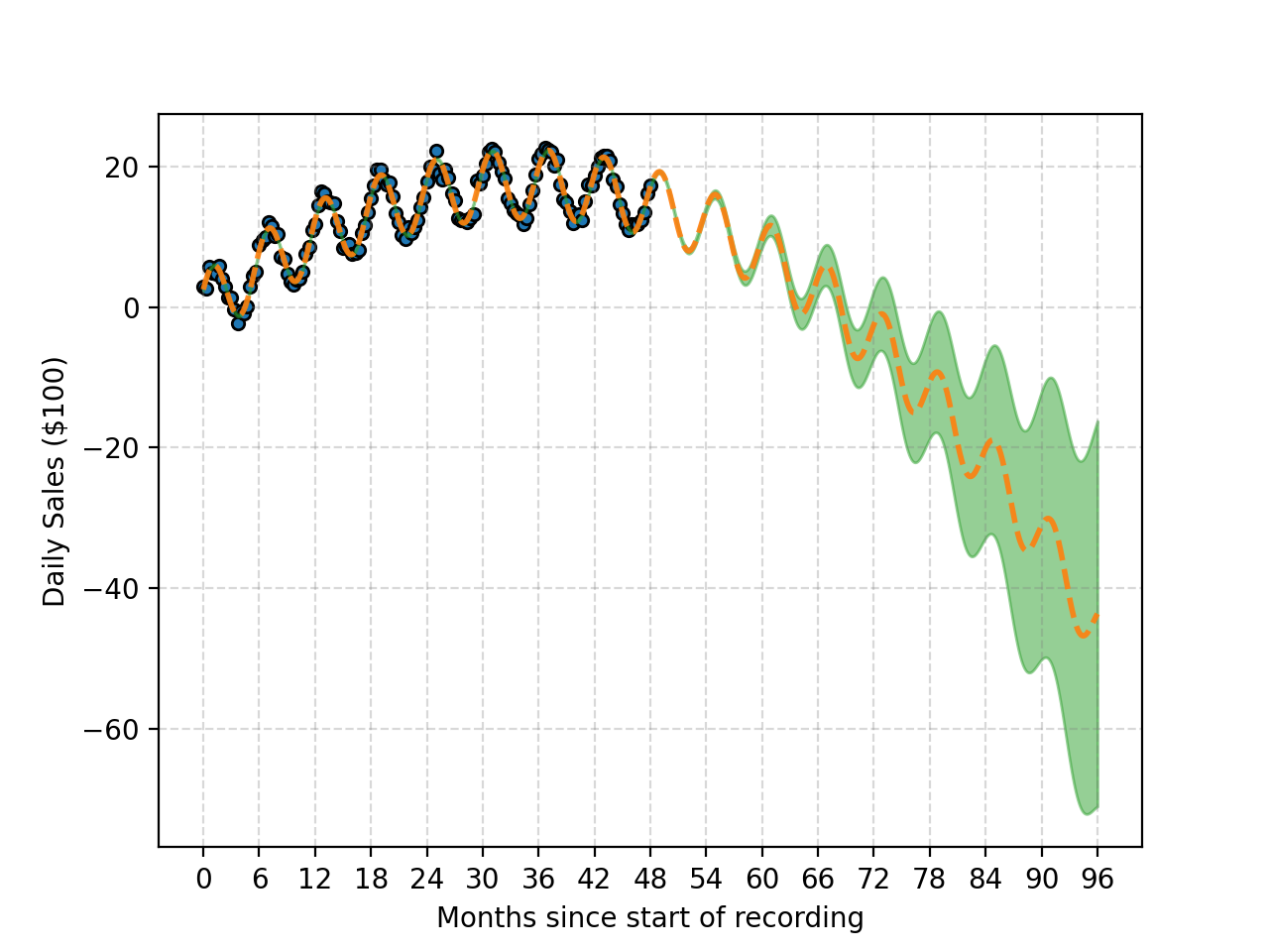
And because we actually know exactly what the curve should look like we can also take a peek at that.

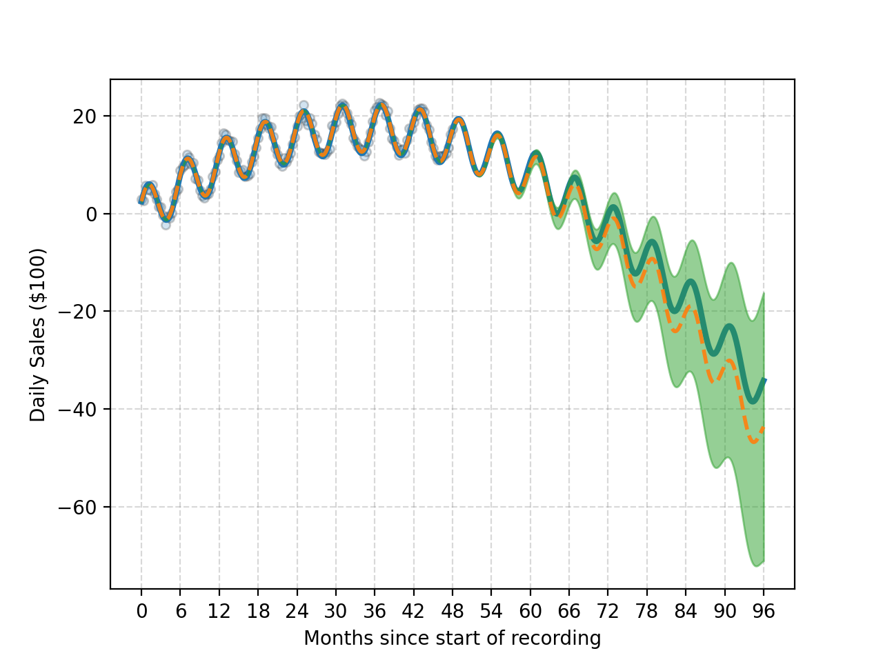
Yay! Seems pretty very good, the exact fit is well contained within the uncertainties but simultaneously the uncertainties don’t look unrealistically large for the data that was given. There’s other more rigorous ways that we could check and see if our prediction is robust/correct but this post is already long enough so I’ll leave this example here.

Gallery of Kernels

Resources

• Interactive Gaussian Process Visualization
• Kernels for Gaussian Processes (blog post) - anders e

More examples of fundamental kernels

We’ve already seen and tried to understand a couple fundamental kernels.

The Exponential Sine Squared or simply periodic kernel that allows us to model periodic behaviour,

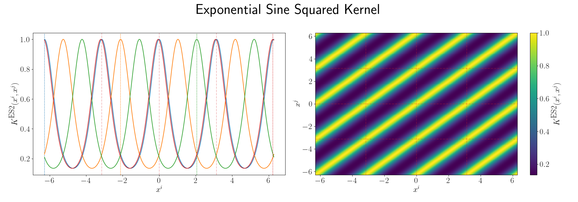
and the RBF or gaussian kernel which allows us to group nearby points together.

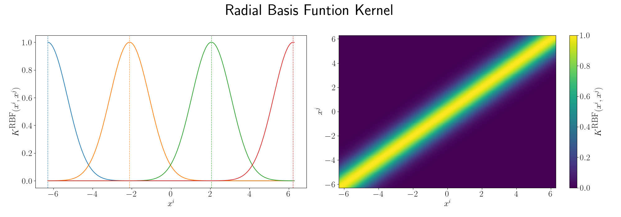
Now let’s look at a few more examples. (Shun Cheung’s blog post on GPs has some nice GIFs about what types of functions actually pop out of these kernels btw.)

Up first is the Laplace Kernel or Matern 1/2 which has the form,

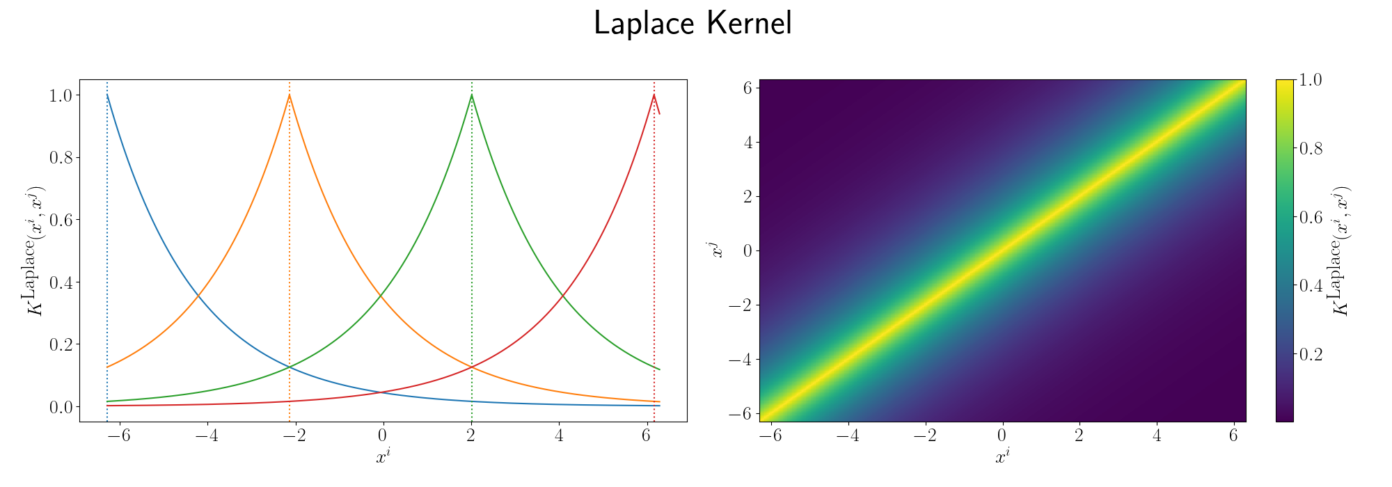
The Chi Squared Kernel has the form,

where \(x_i^k\) is the \(\textrm{k}^{\textrm{th}}\) element of the vector \(x_i\).

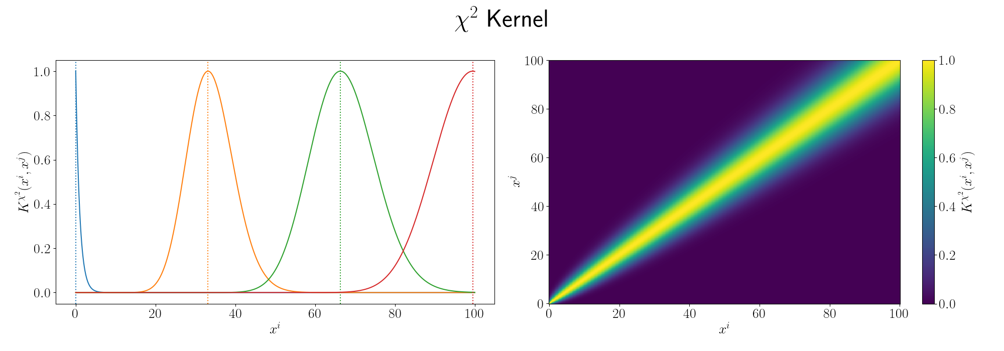
The Sigmoid Kernel has the form,

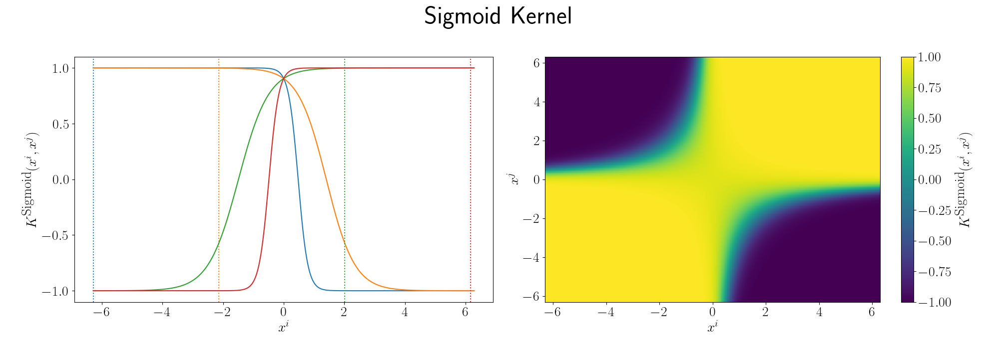
The Matern Kernel has the form,

The White Noise has the following form.

Combining Kernels

I’ve covered most of the basic kernels that people typically use in their work. But, these are more often than not combined with each other to be able to model more specific behaviours by either multiplying or adding the kernels together.

PROMISE I WILL GET TO THIS SOON GO HERE FOR NOW I GUESS

Conclusions / Pros and Cons of Kernel Methods

Alrighty, hopefully I’ve given some introductory view for whatever method you clicked on this post for! If you read the whole thing, you should maybe go outside and touch some grass.

Some (actual) thoughts on these methods:

1. They are often up to cubic in computational complexity in regards to dataset size. (The overheads taking up comp time vary for SVM and KDA for example so sometimes it’s effectively down to quadratic complexity.) So one has to be careful about comp time in cases of very large datasets
2. In the case of data discrimination and classification and high dimensional data the base linear forms of the methods above can perform about as well sometimes for a fraction of the cost (e.g. PCA vs KPCA below, but that is likely because of my haphazard implementation of KPCA).
3. Picking a kernel can be hard, and picking the hyperparameters for those kernels can often be harder e.g. With classification with RBF kernel \(\sigma=0.01\) above could lead to overfitting and \(\sigma=10\) could lead to underfitting.

Among some others that I don’t feel confident in explaining at the moment (Nov 2025). But generally if you’re dataset is small/medium sized with these methods you get nice guarantees about the type of optimisation being perform (if you do optimisation instead of sampling), expressivity and general statistical rigour that machine learning approaches almost always lack. And there are probably many more things that are great about them that I’d love to add here if you have any suggestions.

Overall, I’d highly recommend giving Rasmussen - “Gaussian Processes for Machine Learning” and Steinwart - “Support Vector Machines” (if you have access) for the math around kernel methods.

More Examples

PCA vs KPCA | Facial Recognition

Another famous application of PCA is that of compressing down image data, particularly that of faces. Following the example from the scikit-learn documentation we will try to compare the performance of using PCA vs KPCA for this data.

First we’ll get the data, and compress it with PCA in a similar way to the tutorial linked above.

import matplotlib.pyplot as plt
from scipy.stats import loguniform
import time
import numpy as np

from sklearn.datasets import fetch_lfw_people
from sklearn.decomposition import PCA
from sklearn.metrics import ConfusionMatrixDisplay, classification_report
from sklearn.model_selection import RandomizedSearchCV, train_test_split
from sklearn.preprocessing import StandardScaler
from sklearn.svm import SVC

lfw_people = fetch_lfw_people(min_faces_per_person=141, resize=0.4)

n_samples, h, w = lfw_people.images.shape

X = lfw_people.data
n_features = X.shape[1]

# the label to predict is the id of the person
y = lfw_people.target
target_names = lfw_people.target_names
n_classes = target_names.shape[0]

print("Total dataset size:")
print("n_samples: %d" % n_samples)
print("n_features: %d" % n_features)
print("n_classes: %d" % n_classes)


X_train, X_test, y_train, y_test = train_test_split(
    X, y, test_size=0.1, random_state=42
)

scaler = StandardScaler()
X_train = scaler.fit_transform(X_train)
X_test = scaler.transform(X_test)

I then use less components as initially I thought that KPCA might do better with less as it can construct more complicated projections and thus retain more information for each ‘component’…

n_components = 16

print(
    "Extracting the top %d eigenfaces from %d faces" % (n_components, X_train.shape[0])
)
t0 = time.time()
pca = PCA(n_components=n_components, svd_solver="randomized", whiten=True).fit(X_train)
print("done in %0.3fs" % (time.time() - t0))

eigenfaces = pca.components_.reshape((n_components, h, w))

print("Projecting the input data on the eigenfaces orthonormal basis")
t0 = time.time()
X_train_pca = pca.transform(X_train)
X_test_pca = pca.transform(X_test)
print("done in %0.3fs" % (time.time() - t0))

Then using the projected data X_train_pca and X_test_pca we can train a Support Vector Machine classifier or simply SVC.

from sklearn.experimental import enable_halving_search_cv  # Must include this line
from sklearn.model_selection import HalvingRandomSearchCV
from sklearn.svm import SVC
from scipy.stats import loguniform
import time

print("Fitting the classifier with HalvingRandomSearchCV")
t0 = time.time()
param_distributions = {
    # Keep using loguniform for efficient search on C and gamma
    "C": loguniform(1e1, 1e7),
    "gamma": loguniform(1e-8, 1e1),
}

# The 'n_candidates' here controls the total number of configurations to try
# The 'factor' controls how aggressively configurations are culled (higher = faster but riskier)
clf = HalvingRandomSearchCV(
    estimator=SVC(kernel="rbf", class_weight="balanced", random_state=42),
    param_distributions=param_distributions,
    n_candidates=1000, # Total initial configurations (similar to n_iter=100)
    factor=2,
    cv=5,
    random_state=42
)

clf = clf.fit(X_train_pca, y_train) # Use your actual data here

print("done in %0.3fs" % (time.time() - t0))
print("Best estimator found by HalvingRandomSearchCV:")
print(clf.best_estimator_)

One of the cool things about doing PCA vs KPCA here is that we can directly visualise the components that we are projecting our data on to, i.e. the principle components. Specifically for this data they’re sometimes referred to as ‘eigenfaces’.

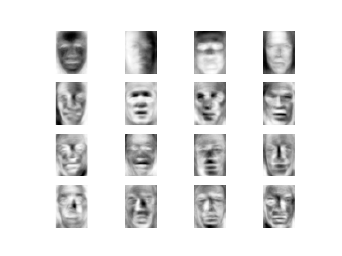
This is pretty close to how the PCA understand the space of pixels and thus the faces we’ve given it. The data is basically a linear combination of these features from the perspective of PCA. We can see that the first few faces are pretty blurry and as you go on they generally add more and more detail.

We can understand this as the first few components that explain most of the variation in our pixel data as: 1. intensity and structure of the average face in the dataset 2.left and right hand side lighting/head angle with a bit more structure and then for 3. up down lighting/head tilt with a bit more structure again.

We then get a pretty good confusion matrix with overall accuracy of 78%.

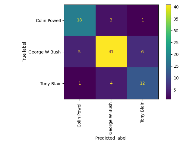
We can then observe what faces were classified as what from the dataset with only 2 mis-identified within the set. And both George Bush, not sure if that means anything.

Now we can attempt to repeat this with Kernel PCA. I’m thinking that since the linear component is doing so well that we will keep a linear kernel component but also maybe try and relate the positions of the image vectors using an RBF kernel.

I arrived on a kernel like this.

from sklearn.metrics.pairwise import linear_kernel, rbf_kernel


def composite_rbf_linear_kernel(X, Y, gamma=1e-3):
    X = np.array([X])
    Y = np.array([Y])

    K_rbf = rbf_kernel(X, Y, gamma=gamma)
    
    K_linear = linear_kernel(X, Y)
    
    
    return K_rbf + K_linear

We do pretty much the exact same projection and classification training.

from sklearn.decomposition import KernelPCA

print(
    "Extracting the top %d eigenfaces from %d faces" % (n_components, X_train.shape[0])
)
t0 = time.time()
kpca = KernelPCA(n_components=n_components, kernel=composite_rbf_linear_kernel, fit_inverse_transform=True).fit(X_train)
print("done in %0.3fs" % (time.time() - t0))

# kpca_eigenfaces = kpca.components_.reshape((n_components, h, w))

print("Projecting the input data on the eigenfaces orthonormal basis")
t0 = time.time()
X_train_kpca = kpca.transform(X_train)
X_test_kpca = kpca.transform(X_test)
print("done in %0.3fs" % (time.time() - t0))


from sklearn.experimental import enable_halving_search_cv  # Must include this line
from sklearn.model_selection import HalvingRandomSearchCV
from sklearn.svm import SVC
from scipy.stats import loguniform
import time

print("Fitting the classifier with HalvingRandomSearchCV")
t0 = time.time()
param_distributions = {
    # Keep using loguniform for efficient search on C and gamma
    "C": loguniform(1e1, 1e7),
    "gamma": loguniform(1e-8, 1e1),
}

# The 'n_candidates' here controls the total number of configurations to try
# The 'factor' controls how aggressively configurations are culled (higher = faster but riskier)
clf_kpca = HalvingRandomSearchCV(
    estimator=SVC(kernel="rbf", class_weight="balanced", random_state=42),
    param_distributions=param_distributions,
    n_candidates=2000, # Total initial configurations (similar to n_iter=100)
    factor=3,
    cv=5,
    random_state=42
)

clf_kpca = clf_kpca.fit(X_train_kpca, y_train) # Use your actual data here

print("done in %0.3fs" % (time.time() - t0))
print("Best estimator found by HalvingRandomSearchCV:")
print(clf_kpca.best_estimator_)

We cannot directly view the eigenfaces here as we have projected the data into a much higher dimensional space again with our non-linear components so it does make immediate sense to even try looking at them in the same way as we did for PCA.

But we did get the embedded values from the KPCA and put that through the classifier, so let’s have a look at how well the same classifier did with the KPCA embedding/summary/components.

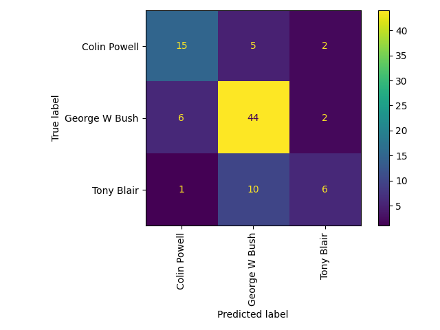
Not that much worse than PCA, but still notably worse with an overall accuracy of 70%. Now let’s have a glance at the classification results for different inputs.

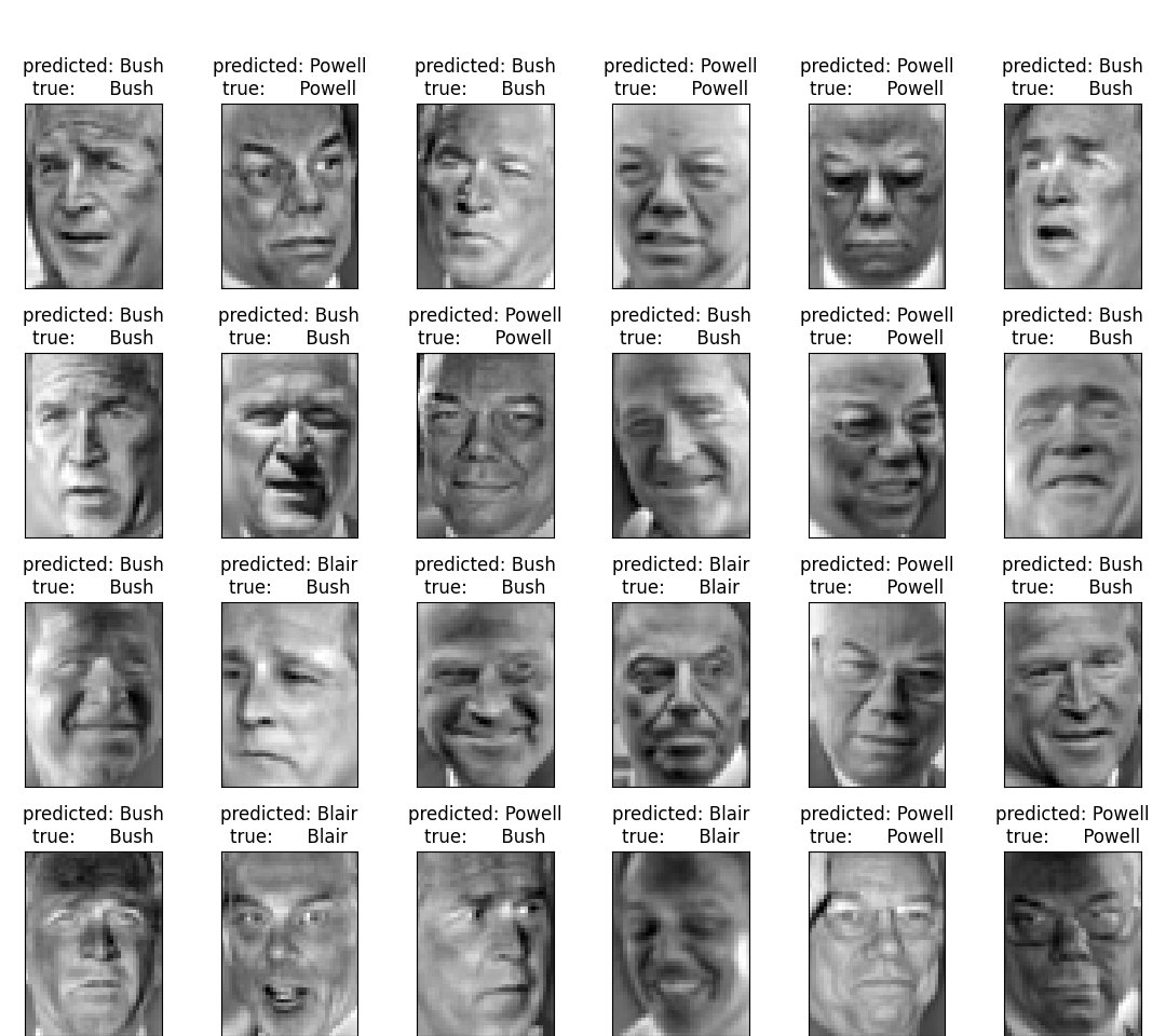
And we miss the same faces! Damn George Bush(‘s face). So these might be an aspect of the data that are particularly hard to distinguish. Notably both are at pretty extreme facial angles so maybe that’s it.

So the KPCA did worse. This may be because we were more likely to fit to noise/random artefacts (although I did try and regularise and deregularise the KPCA projection), or inability to find a good set of parameters for the classifier, or the mere fact that I didn’t optimise for the parameters of the KPCA kernel, or a vast number of things due to my insufficient amount of time to really do everything robustly. In my opinion it’s likely the fact that I didn’t optimise for the KPCA kernel parameters or that the classifier doesn’t match up as well with KPCA as it does with PCA, so it might be interesting to see if using different classifier architectures retain the same behaviour. I might tackle this in a later post but for now I’ll leave it here.